Exercise 3.7: Comparison of Two Convolutional Encoders
From LNTwww
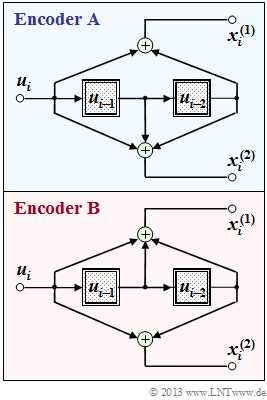
The graph shows two rate $1/2$ convolutional encoders, each with memory $m = 2$:
- The encoder $\rm A$ has the transfer function matrix $\mathbf{G}(D) = (1 + D^2, \ 1 + D + D^2)$.
- In encoder $\rm B$ the two filters $($top and bottom$)$ are interchanged, and it holds:
- $$\mathbf{G}(D) = (1 + D + D^2, \ 1 + D^2).$$
The lower encoder $\rm B$ has already been treated in detail in the theory part.
In the present exercise,
- you are first to determine the state transition diagram for encoder $\rm A$,
- and then work out the differences and the similarities between the two state diagrams.
Hints:
- This exercise belongs to the chapter "Code description with state and trellis diagram".
- Reference is made in particular to the sections
Questions
Solution
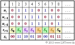
(1) The calculation is based on the equations
- $$x_i^{(1)} = u_i + u_{i–2},$$
- $$x_i^{(2)} = u_i + u_{i–1} + u_{i–2}.$$
- Initially, the two memories $(u_{i–1}$ and $u_{i–2})$ are preallocated with zeros ⇒ $s_1 = S_0$.
- With $u_1 = 0$, we get $\underline{x}_1 = (00)$ and $s_2 = S_0$.
- With $u_2 = 1$, one obtains the output $\underline{x}_2 = (11)$ and the new state $s_3 = S_3$.
From the adjacent calculation scheme one recognizes the correctness of the proposed solutions 1 and 4.
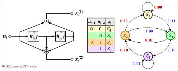
(2) All proposed solutions are correct:
- This can be seen by evaluating the table at subtask (1).
- The results are shown in the adjacent graph.
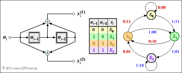
(3) Correct is only statement 3:
- The state transition diagram of encoder $\rm B$ is sketched on the right. For derivation and interpretation, see section "Representation in the state transition diagram".
- If we swap the two output bits $x_i^{(1)}$ and $x_i^{(2)}$, we get from the convolutional encoder $\rm A$ to the convolutional encoder $\rm B$ $($and vice versa$)$.


