Code Description with State and Trellis Diagram

State definition for a memory register

A convolutional encoder can also be understood as an automaton with a finite number of states. This number results from the number $m$ of memory elements to $2^m$.

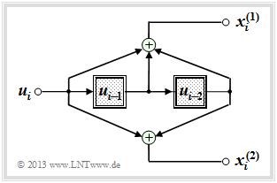
In this chapter we mostly start from the drawn convolutional encoder, which is characterized by the following parameters:

Convolutional encoder with $k = 1, \ n = 2, \ m = 2$

$k = 1, \ n = 2$ ⇒ code rate $R = 1/2$,

Memory $m = 2$ ⇒ influence length $\nu = m+1=3$,

Transfer function matrix in octal form $(7, 5)$:

$$\mathbf{G}(D) = (1 + D + D^2, \ 1 + D^2).$$

The encoded sequence $\underline{x}_i = (x_i^{(1)}, \ x_i^{(2)})$ at time $i$ depends not only on the information bit $u_i$ but also on the content $(u_{i-1}, \ u_{i-2})$ of the memory.

There are $2^m = 4$ possibilities for this, namely the states $S_0, \ S_1, \ S_2,\ S_3$.

Let the register state $S_{\mu}$ be defined by the index

\[\mu = u_{i-1} + 2 \cdot u_{i-2}\hspace{0.05cm}, \hspace{0.5cm}{\rm general\hspace{-0.1cm}:}\hspace{0.15cm} \mu = \sum_{l = 1}^{m} \hspace{0.1cm}2\hspace{0.03cm}^{l-1} \cdot u_{i-l} \hspace{0.05cm}.\]

To avoid confusion, we distinguish in the following by upper or lower case letters:

the possible states $S_{\mu}$ with the indices $0 ≤ \mu ≤ 2^m \,-1$,
the current states $s_i$ at the times $i = 1, \ 2, \ 3, \ \text{...}$

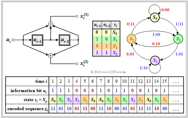
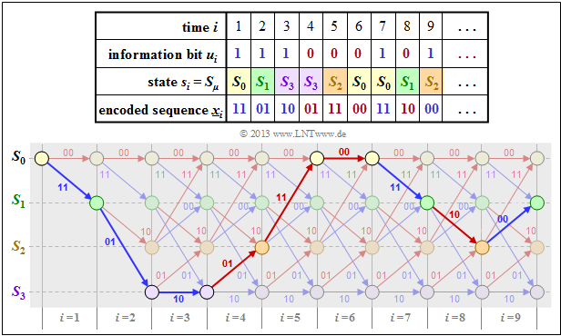
$\text{Example 1:}$ The graph shows for the convolutional encoder sketched above

To illustrate the states $S_{\mu}$

the information sequence $\underline{u} = (u_1,u_2, \text{...} \ ) $
⇒ information bits $u_i$,

the current states at times $i$
⇒ $s_i ∈ \{S_0, \ S_1, \ S_2, \ S_3\}$,

the 2–bit sequences $\underline{x}_i = (x_i^{(1)}, \ x_i^{(2)})$
⇒ encoding the information bit $u_i$.

For example, you can see from this illustration $($the colors are to facilitate the transition to later graphics$)$:

At time $i = 5$ ⇒ $u_{i-1} = u_4 = 0$, $u_{i-2} = u_3 = 1$ holds. That is, the automat is in state $s_5 = S_2$.
With the information bit $u_i = u_5 = 0$, the encoded sequence $\underline{x}_5 = (11)$ is obtained.
The state for time $i = 6$ results from $u_{i-1} = u_5 = 0$ and $u_{i-2} = u_4 = 0$ to $s_6 = S_0$.
Because of $u_6 = 0$ ⇒ $\underline{x}_6 = (00)$ is output and the new state $s_7$ is again $S_0$.
At time $i = 12$ the encoded sequence $\underline{x}_{12} = (11)$ is output because of $u_{12} = 0$ as at time $i = 5$.
Here, one passes from state $s_{12} = S_2$ to state $s_{13} = S_0$ .
In contrast, at time $i = 9$ the encoded sequence $\underline{x}_{9} = (00)$ is output and state $s_9 = S_2$ is followed by $s_{10} = S_1$.
The same is true for $i = 15$. In both cases, the current information bit is $u_i = 1$.

$\text{Conclusion:}$ From this example it can be seen that the encoded sequence $\underline{x}_i$ at time $i$ depends solely on

the current state $s_i = S_{\mu} \ (0 ≤ \mu ≤ 2^m -1)$, as well as
the current information bit $u_i$.

Similarly, the successor state $s_{i+1}$ is determined by $s_i$ and $u_i$ alone.

These properties are considered in the so-called "state transition diagram" in the next section.

Representation in the state transition diagram

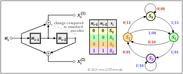
The graph shows the state transition diagram for the $(n = 2, \ k = 1, \ m = 2)$ convolutional encoder.

State transition diagram $\rm A$ for the $(n = 2, \ k = 1, \ m = 2)$ convolutional encoder;
in the following: "our standard convolutional encoder"

This diagram provides all information about this special convolutional encoder in compact form.
The color scheme is aligned with the $\text{sequential representation}$ in the previous section.
For the sake of completeness, the derivation table is also given again.
The $2^{m+k}$ transitions are labeled "$u_i \ | \ \underline{x}_i$".

For example, it can be read:

The information bit $u_i = 0$ $($indicated by a red label$)$ takes you from state $s_i = S_1$ to state $s_{i+1} = S_2$ and the two code bits are $x_i^{(1)} = 1, \ x_i^{(2)} = 0$.

With the information bit $u_i = 1$ $($blue label$)$ in the state $s_i = S_1$ the code bits result in $x_i^{(1)} = 0, \ x_i^{(2)} = 1$, and one arrives at the new state $s_{i+1} = S_3$.

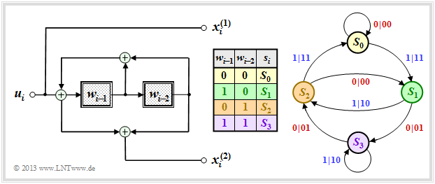
State transition diagram $\rm B$ for another $(n = 2, \ k = 1, \ m = 2)$ convolutional encoder;
in the following: "equivalent systematic representation"

We now consider another systematic encoder with same parameters:

$$n = 2, \ k = 1, \ m = 2.$$

This is the $\text{equivalent systematic representation}$ of our standard convolutional encoder, also referred to as "recursive systematic convolutional encoder".

Compared to the upper state transition diagram $\rm A$, one can see the following differences:

Since the earlier information bits $u_{i-1}$ and $u_{i-2}$ are not stored, here the states $s_i = S_{\mu}$ are related to the processed quantities $w_{i-1}$ and $w_{i-2}$, where $w_i = u_i + w_{i-1} + w_{i-2}$ holds.

Since this code is also systematic ⇒ $x_i^{(1)} = u_i$. The derivation of the second code bits $x_i^{(2)}$ can be found in "Exercise 3.5". It is a recursive filter, as described in the "Filter structure with fractional–rational transfer function" section.

$\text{Conclusion:}$ The comparison of the graphics shows that a similar state transition diagram is obtained for both encoders:

The structure of the state transition diagram is determined solely by the parameters $m$ and $k$ .

The number of states is $2^{m \hspace{0.05cm}\cdot \hspace{0.05cm}k}$ and $2^k$ arrows go from each state.

You also get from each state $s_i ∈ \{S_0, \ S_1, \ S_2, \ S_3\}$ to the same successor states $s_{i+1}$.

A difference exists solely with respect to the encoded sequences output, where in both cases $\underline{x}_i ∈ \{00, \ 01, \ 10, \ 11\}$ applies.

Representation in the trellis diagram

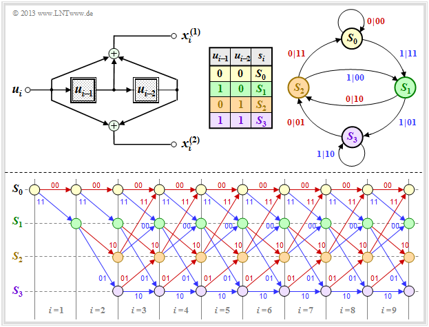
One gets from the state transition diagram to the so-called "trellis diagram" $($short: $\text{trellis)}$ by additionally considering a time component ⇒ control variable $i$. The following graph contrasts both diagrams for "our standard convolutional encoder". The bottom illustration has a resemblance to a "garden trellis" – assuming some imagination.

State transition diagram vs. trellis diagram for "our standard convolutional encoder"

Further is to be recognized on the basis of this diagram:

Since all memory registers are preallocated with zeros, the trellis always starts from the state $s_1 = S_0$. At the next time $(i = 2)$ only the two states $S_0$ and $S_1$ are possible.
From time $i = m + 1 = 3$ the trellis has exactly the same appearance for each transition from $s_i$ to $s_{i+1}$. Each state $S_{\mu}$ is connected to a successor state by a red arrow $(u_i = 0)$ and a blue arrow $(u_i = 1)$.
Versus a "code tree" that grows exponentially with each time step $i$ – see for example section "Error sizes and total error sizes" in the book "Digital Signal Transmission" – here the number of nodes $($i.e. possible states$)$ is limited to $2^m$ .
This pleasing property of any trellis diagram is also used by the $\text{Viterbi algorithm}$ for efficient maximum likelihood decoding of convolutional codes.

The following example is to show that there is a "$1\text{:}1$" mapping between the string of encoded sequences $\underline{x}_i$ and the paths through the trellis diagram.

Also the information sequence $\underline{u}$ can be read from the selected trellis path based on the colors of the individual branches.

A red branch stands for the information bit $u_i = 0$, a blue one for $u_i = 1$.

$\text{Example 2:}$ In the former $\text{Example 1}$ the encoded sequence $\underline{x}$ was derived

for our rate $1/2$ standard convolutional encoder with memory $m = 2$ and

the information sequence $\underline{u} = (1, 1, 1, 0, 0, 0, 1, 0, 1, \ \text{. ..})$

Trellis diagram of a sample sequence

The table on the right shows the result for $i ≤ 9$ once again. The trellis diagram is drawn below. You can see:

The selected path through the trellis is obtained by lining up red and blue arrows representing the possible information bits $u_i \in \{ 0, \ 1\}$ .
This statement is true for any rate $1/n$ convolutional code. For a code with $k > 1$ there would be $2^k$ different colored arrows.
For a rate $1/n$ convolutional code, the arrows are labeled with the code words $\underline{x}_i = (x_i^{(1)}, \ \text{...} \ , \ x_i^{(n)})$ which are derived from the information bit $u_i$ and the current register states $s_i$.
For $n = 2$ there are only four possible code words, namely $00, \ 01, \ 10$ and $11$.
In vertical direction, one recognizes from the trellis the register states $S_{\mu}$. Given a rate $k/n$ convolutional code with memory order $m$ there are $2^{k \hspace{0.05cm}\cdot \hspace{0.05cm}m}$ different states.
In the present example $(k = 1, \ m = 2)$ these are the states $S_0, \ S_1, \ S_2$ and $S_3$.

Definition of the free distance

An important parameter of linear block codes is the $\text{minimum Hamming distance}$ between any two code words $\underline{x}$ and $\underline{x}\hspace{0.05cm}'$:

\[d_{\rm min}(\mathcal{C}) = \min_{\substack{\underline{x},\hspace{0.05cm}\underline{x}' \hspace{0.05cm}\in \hspace{0.05cm} \mathcal{C} \\ {\underline{x}} \hspace{0.05cm}\ne \hspace{0.05cm} \underline{x}\hspace{0.03cm}'}}\hspace{0.1cm}d_{\rm H}(\underline{x}, \hspace{0.05cm}\underline{x}\hspace{0.03cm}')\hspace{0.05cm}.\]

Due to linearity, the zero word $\underline{0}$ also belongs to each block code. Thus $d_{\rm min}$ is identical to the minimum $\text{Hamming weight}$ $w_{\rm H}(\underline{x})$ of a code word $\underline{x} ≠ \underline{0}$.

For convolutional codes, however, the description of the distance ratios proves to be much more complex, since a convolutional code consists of infinitely long and infinitely many encoded sequences. Therefore we define here instead of the minimum Hamming distance:

$\text{Definition:}$

The »free distance« $d_{\rm F}$ of a convolutional code is equal to the number of bits in which any two encoded sequences $\underline{x}$ and $\underline{x}\hspace{0.03cm}' $ differ $($at least$)$.

In other words: The free distance is equal to the minimum Hamming distance between any two paths through the trellis.

Since convolutional codes are linear, we can also use the infinite zero sequence as a reference sequence: $\underline{x}\hspace{0.03cm}' = \underline{0}$. Thus, the free distance $d_{\rm F}$ is equal to the minimum Hamming weight $($number of "ones"$)$ of a encoded sequence $\underline{x} ≠ \underline{0}$.

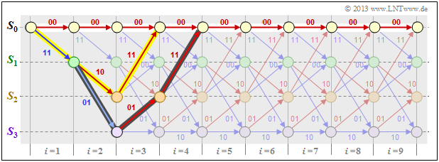
$\text{Example 3:}$ We consider the null sequence $\underline{0}$ (marked with white filled circles) as well as two other encoded sequences $\underline{x}$ and $\underline{x}\hspace{0.03cm}'$ (with yellow and dark background, respectively) in our standard trellis and characterize these sequences based on the state sequences:

On the definition of free distance

$$\underline{0} =\left ( S_0 \rightarrow S_0 \rightarrow S_0\rightarrow S_0\rightarrow S_0\rightarrow \hspace{0.05cm}\text{...} \hspace{0.05cm}\right)$$

$$\hspace{0.3cm} \Rightarrow \hspace{0.3cm} \underline{0} = \left ( 00, 00, 00, 00, 00,\hspace{0.05cm} \text{...} \hspace{0.05cm}\right) \hspace{0.05cm},$$

$$\ \underline{x} =\left ( S_0 \rightarrow S_1 \rightarrow S_2\rightarrow S_0\rightarrow S_0\rightarrow \hspace{0.05cm}\text{...} \hspace{0.05cm}\right)$$

$$\hspace{0.3cm} \Rightarrow \hspace{0.3cm}\underline{x} == \left ( 11, 10, 11, 00, 00,\hspace{0.05cm} \text{...} \hspace{0.05cm}\right) \hspace{0.05cm},$$

$$\underline{x}\hspace{0.03cm}' = \left ( S_0 \rightarrow S_1 \rightarrow S_3\rightarrow S_2\rightarrow S_0\rightarrow \hspace{0.05cm}\text{...} \hspace{0.05cm}\right)$$

$$\hspace{0.3cm} \Rightarrow \hspace{0.3cm}\underline{x}\hspace{0.03cm}' = \left ( 11, 01, 01, 11, 00,\hspace{0.05cm} \text{...} \hspace{0.05cm}\right) \hspace{0.05cm}.$$

One can see from these plots:

The free distance $d_{\rm F} = 5$ is equal to the Hamming weight $w_{\rm H}(\underline{x})$.
No sequence other than the one highlighted in yellow differs from $\underline{0}$ by less than five bits. For example $w_{\rm H}(\underline{x}') = 6$.
In this example, the free distance $d_{\rm F} = 5$ also results as the Hamming distance between the sequences $\underline{x}$ and $\underline{x}\hspace{0.03cm}'$, which differ in exactly five bit positions.

The larger the free distance $d_{\rm F}$, the better is the "asymptotic behavior" of the convolutional encoder.

For the exact error probability calculation, however, one needs the exact knowledge of the $\text{weight enumerator function}$ just as for the linear block codes.

This is given for the convolutional codes in detail only in the chapter "Distance Characteristics and Error Probability Bounds".

Optimal convolutional codes of rate $1/2$

At the outset, just a few remarks:

The free distance $d_{\rm F}$ increases with increasing memory $m$ provided that one uses appropriate polynomials for the transfer function matrix $\mathbf{G}(D)$ .
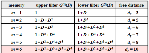
In the table for rate $1/2$ convolutional codes, the $n = 2$ polynomials are given together with the $d_{\rm F}$ value.
Of greater practical importance is the "industry standard code" with $m = 6$ ⇒ $64$ states and the free distance $d_{\rm F} = 10$ $($in the table this is highlighted in red$)$.

The following example shows the effects of using unfavorable polynomials.

$\text{Example 4:}$ In $\text{Example 3}$ it was shown that our standard convolutional encoder $(n = 2, \ k = 1, \ m = 2)$ has the free distance $d_{\rm F} = 5$. This is based on the transfer function matrix $\mathbf{G}(D) = (1 + D + D^2, \ 1 + D^2)$, as shown in the model $($without red deletion$)$.

State transition diagram $\rm C$ for the modified standard convolutional encoder

Using $\mathbf{G}(D) = (1 + D, \ 1 + D^2)$ ⇒ red change, the state transition diagram changes from the $\text{state transition diagram $\rm A$}$ little at first glance. However, the effects are serious:

The free distance is no longer $d_{\rm F} = 5$, but $d_{\rm F} = 3$, where the encoded sequence $\underline{x} = (11, \ 01, \ 00, \ 00, \text{. ..})$ with only three ones belonging to the information sequence $\underline{u} = \underline{1} = (1, \ 1, \ 1, \ 1, \ \text{...})$.
That is: By only three transmission errors at positions 1, 2, and 4, one falsifies the "one sequence" $(\underline{1})$ into the "zero sequence" $(\underline{0})$ and thus produces infinitely many decoding errors in state $S_3$.
A convolutional encoder with these properties is called "catastrophic". The reason for this extremely unfavorable behavior is that here the two polynomials $1 + D$ and $1 + D^2$ are not divisor-remote.

Terminated convolutional codes

In the theoretical description of convolutional codes, one always assumes information sequences $\underline{u}$ and encoded sequences $\underline{x}$ that are by definition infinite in length.

On the other hand, in practical applications e.g. $\text{GSM}$ and $\text{UMTS}$, one always uses an information sequence of finite length $L$.

For a rate $1/n$ convolutional code, the encoded sequence then has at least length $n \cdot L$.

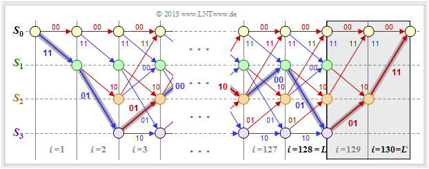
The graph $($without the gray background$)$ shows the trellis of our standard rate $1/2$ convolutional code at binary input sequence $\underline{u}$ of finite length $L = 128$.

Terminated convolutional code of rate $R = 128/260$

Thus the encoded sequence $\underline{x}$ has length $2 \cdot L = 256$.

However, due to the undefined final state, a complete maximum likelihood decoding of the transmitted sequence is not possible.

Since it is not known which of the states $S_0, \ \text{...} \ , \ S_3$ would occur for $i > L$, the error probability will be $($somewhat$)$ larger than in the limiting case $L → ∞$.

To prevent this, the convolutional code is terminated as shown in the diagram: You add $m = 2$ zeros to the $L = 128$ information bits ⇒ $L' = 130$.

This results, for example, for the color highlighted path through the trellis:

$$\underline{x}' = (11\hspace{0.05cm},\hspace{0.05cm} 01\hspace{0.05cm},\hspace{0.05cm} 01\hspace{0.05cm},\hspace{0.05cm} 00 \hspace{0.05cm},\hspace{0.05cm} \text{...}\hspace{0.1cm},\hspace{0.05cm} 10\hspace{0.05cm},\hspace{0.05cm}00\hspace{0.05cm},\hspace{0.05cm} 01\hspace{0.05cm},\hspace{0.05cm} 01\hspace{0.05cm},\hspace{0.05cm} 11 \hspace{0.05cm} ) $$

$$\Rightarrow \hspace{0.3cm}\underline{u}' = (1\hspace{0.05cm},\hspace{0.05cm} 1\hspace{0.05cm},\hspace{0.05cm} 0\hspace{0.05cm},\hspace{0.05cm} 1 \hspace{0.05cm},\hspace{0.05cm} \text{...}\hspace{0.1cm},\hspace{0.05cm} 0\hspace{0.05cm},\hspace{0.05cm}1\hspace{0.05cm},\hspace{0.05cm} 1\hspace{0.05cm},\hspace{0.05cm} 0\hspace{0.05cm},\hspace{0.05cm} 0 \hspace{0.05cm} ) \hspace{0.05cm}.$$

The trellis now ends always $($independent of the data$)$ in the defined final state $S_0$; one thus achieves the best possible error probability according to maximum likelihood.

However, the improvement in error probability comes at the cost of a lower code rate.

For $L \gg m$ this loss is only small. In the considered example, instead of $R = 0.5$ with termination the code rate results in

$$R\hspace{0.05cm}' = 0.5 \cdot L/(L + m) \approx 0.492.$$

Punctured convolutional codes

$\text{Definition:}$

We assume a convolutional code of rate $R_0 = 1/n_0$ which we call "mother code".

If one deletes some bits from its encoded sequence according to a given pattern, it is called a »punctured convolutional code« with code rate $R > R_0$.

The puncturing is done using the puncturing matrix $\mathbf{P}$ with the following properties:

The row number is $n_0$, the column number is equal to the puncturing period $p$, which is determined by the desired code rate.
The $n_0 \cdot p$ matrix elements $P_{ij}$ are binary $(0$ or $1)$.
If $P_{ij} = 1$ the corresponding code bit $x_{ij}$ is taken, if $P_{ij} = 0$ not.
The rate of the punctured code is equal to the quotient of the puncturing period $p$ and the number $N_1$ of ones in the $\mathbf{P}$ matrix.

One can usually find favorably punctured convolutional codes only by means of computer-aided search. Here, a punctured convolutional code is said to be favorable if it has

the same memory order $m$ as the parent code, and also the total influence length is the same in both cases: $\nu = m + 1$,

a free distance $d_{\rm F}$ as large as possible which is of course smaller than that of the mother code.

$\text{Example 5:}$ Starting from our $\text{rate 1/2 standard code}$ with parameters $n_0 = 2$ and $m = 2$, we obtain with the puncturing matrix

\[{\boldsymbol{\rm P} } = \begin{pmatrix} 1 & 1 & 0 \\ 1 & 0 & 1 \end{pmatrix}\hspace{0.3cm}\Rightarrow \hspace{0.3cm} p = 3\hspace{0.05cm}, \hspace{0.2cm}N_1 = 4\]

a punctured convolutional code of rate $R = p/N_1 = 3/4$.

We consider the following constellation for this purpose:

Information sequence: $\hspace{2.5cm} \underline{u} = (1, 0, 0, 1, 1, 0, \ \text{...}\hspace{0.03cm})$,
encoded sequence without puncturing: $\hspace{0.35cm} \underline{x} = (11, 1 \color{grey}{0}, \color{gray}{1}1, 11, 0\color{gray}{1}, \color{gray}{0}1, \ \text{...}\hspace{0.03cm})$,
encoded sequence with puncturing: $\hspace{0.90cm} \underline{x}\hspace{0.05cm}' = (11, 1\_, \_1, 11, 0\_, \_1, \ \text{...}\hspace{0.03cm})$,
received sequence without errors: $\hspace{0.58cm} \underline{y} = (11, 1\_, \_1, 11, 0\_, \_1, \ \text{...}\hspace{0.03cm})$,
modified received sequence: $\hspace{1.4cm} \underline{y}\hspace{0.05cm}' = (11, 1\rm E, E1, 11, 0E, E1, \ \text{...}\hspace{0.03cm})$.

Note:

So each punctured bit in the received sequence $\underline{y}$ $($marked by an underscore$)$ is replaced by an "Erasure" $\rm (E)$, see "Binary Erasure Channel".

Such an erasure created by the puncturing is treated by the decoder in the same way as an erasure by the channel.

Of course, the puncturing increases the error probability. This can already be seen from the fact that the free distance decreases to $d_{\rm F} = 3$ after the puncturing.

In contrast, the mother code has the free distance $d_{\rm F} = 5$.

For example, puncturing is used in the so-called $\text{RCPC codes}$ $($"rate compatible punctured convolutional codes"$)$. More about this in "Exercise 3.8".