Exercise 5.5Z: ACF after 1st Order Filter
From LNTwww
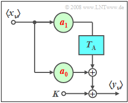
We consider here a first order non-recursive filter $(M = 1)$.
- Let the filter coefficients be $a_0 = 0.4$ and $a_1 = 0.3$.
- A constant $K$ is added at the filter output, which is to be set to zero up to and including subtask (3).
The individual elements of the input sequence $\left\langle \hspace{0.05cm}{x_\nu } \hspace{0.05cm}\right\rangle$
- are Gaussian as well as mean-free, and
- have in each case the standard deviation $\sigma_x = 1$.
Notes:
- The exercise belongs to the chapter Creation of Predefined ACF Properties.
- Reference is also made to the chapters Auto-Correlation Function and Power-Spectral Density.
Questions
Solution
(1) Solutions 2 and 3 are correct:
- The ACF value $\varphi_y(0)$ gives the variance ("power") $\sigma_y^2$ and not the "standard deviation" $\sigma_y$.
- Since a first-order non-recursive filter is present, all ACF values are $\varphi_y(k \cdot T_{\rm A})= 0$ for $|k| \ge 2$.
- The ACF value $\varphi_y(- T_{\rm A})$ is equal to $\varphi_y(+ T_{\rm A})$.
- These two ACF values result in a cosine function in the power-spectral density, to which the DC component $\varphi_y(0)$ is added.
(2) The general equation with $M = 1$ for $k \in \{0, \ 1\}$ is:
- $$\varphi _y ( {k \cdot T_{\rm A} } ) = \sigma _x ^2 \cdot \sum\limits_{\mu = 0}^{M - k} {a_\mu \cdot a_{\mu + k} } .$$
- From this we obtain with $\sigma_x = 1$:
- $$\varphi _y( 0 ) = a_0 ^2 + a_1 ^2 = 0.4^2 + 0.3^2 \hspace{0.15cm}\underline { = 0.25},$$
- $$\varphi _y ( { T_{\rm A} } ) = a_0 \cdot a_1 = 0.4 \cdot 0.3 \hspace{0.15cm}\underline {= 0.12}.$$
(3) With the previous settings, the variance is $\sigma_y^2 = 0.25$ and thus the standard deviation $\sigma_y = 0.5$.
- Doubling the coefficients gives $\sigma_y = 1$ as desired:
- $$\hspace{0.15cm}\underline {a_0 = 0.8},\quad \hspace{0.15cm}\underline {a_1 = 0.6}.$$
(4) The constant $K$ raises the total ACF by $K^2$. Using the result from (2), it follows:
- $$K^2 = 0.5 - 0.25 = 0.25\quad \Rightarrow \quad \hspace{0.15cm}\underline {K = 0.5}.$$
(5) All ACF values are now larger by the constant value $K^2 = 0.25$. Thus
- $$\varphi _y ( { T_{\rm A} } ) = 0.12 + 0.25 \hspace{0.15cm}\underline {= 0.37},$$
- $$\varphi _y ( { 2T_{\rm A} } ) = 0 + 0.25 \hspace{0.15cm}\underline {= 0.25}.$$
(6) The constant $K$ does not change the standard deviation, i.e. $\sigma_y = 0.5$ is still valid.
- Formally, this quantity can also be calculated as follows:
- $$\sigma _y ^2 = \varphi _y ( 0 ) - \mathop {\lim }\limits_{k \to \infty } \varphi _y ( {k \cdot T_{\rm A} } ) = 0.5 - 0.25 = 0.25.$$
- Again, this gives $\sigma_y \hspace{0.15cm}\underline {= 0.5}$.
