Symbolwise Coding with Pseudo-Ternary Codes

General description of the pseudo-multilevel codes

In symbolwise coding, each incoming source symbol $q_\nu$ generates an encoder symbol $c_\nu$, which depends not only on the current input symbol $q_\nu$ but also on the $N_{\rm C}$ preceding symbols $q_{\nu-1}$, ... , $q_{\nu-N_{\rm C}} $. $N_{\rm C}$ is referred to as the "order" of the code.

Typical for symbolwise coding is that

the symbol duration $T$ of the encoded signal (and of the transmitted signal) matches the bit duration $T_{\rm B}$ of the binary source signal, and

encoding and decoding do not lead to major time delays, which are unavoidable when block codes are used.

The "pseudo-multilevel codes" – better known as "partial response codes" – are of special importance. In the following, only "pseudo-ternary codes" ⇒ level number $M = 3$ are considered.

These can be described by the block diagram corresponding to the left graph.
In the right graph an equivalent circuit is given, which is very suitable for an analysis of these codes.

Block diagram (above) and equivalent circuit (below) of a pseudo-ternary encoder

One can see from the two representations:

The pseudo-ternary encoder can be split into the "non-linear pre-encoder" and the "linear coding network", if the delay by $N_{\rm C} \cdot T$ and the weighting by $K_{\rm C}$ are drawn twice for clarity – as shown in the right equivalent figure.

The "non-linear pre-encoder" obtains the precoded symbols $b_\nu$, which are also binary, by a modulo–2 addition ("antivalence") between the symbols $q_\nu$ and $K_{\rm C} \cdot b_{\nu-N_{\rm C}} $:

$$q_\nu \in \{-1, +1\},\hspace{0.1cm} K_{\rm C} \in \{-1, +1\}\hspace{0.3cm}\Rightarrow \hspace{0.3cm}b_\nu \in \{-1, +1\}\hspace{0.05cm}.$$

Like the source symbols $q_\nu$, the symbols $b_\nu$ are statistically independent of each other. Thus, the pre-encoder does not add any redundancy. However, it allows a simpler realization of the decoder and prevents error propagation after a transmission error.

The actual encoding from binary $(M_q = 2)$ to ternary $(M = M_c = 3)$ is done by the "linear coding network" by the conventional subtraction

$$c(t) ={1}/{2} \cdot \big [b(t) - K_{\rm C} \cdot b(t- N_{\rm C}\cdot T)\big] \in \{-1, \ 0, +1\}\hspace{0.05cm},$$

which can be described by the following "impulse response" resp. "transfer function" with respect to the input signal $b(t)$ and the output signal $c(t)$:

$$h_{\rm C}(t) = {1}/{2} \cdot \big [\delta(t) - K_{\rm C} \cdot \delta(t- N_{\rm C}\cdot T)\big] \ \ \ \circ\!\!-\!\!\!-\!\!\!-\!\!\bullet\ \ \ H_{\rm C}(f) ={1}/{2} \cdot \left [1 - K_{\rm C} \cdot {\rm e}^{- {\rm j}\hspace{0.05cm}\cdot\hspace{0.05cm} 2\pi \hspace{0.05cm}\cdot \hspace{0.05cm}N_{\rm C}\hspace{0.05cm}\cdot \hspace{0.05cm}T}\right]\hspace{0.05cm}. $$

The relative redundancy is the same for all pseudo-ternary codes. Substituting $M_q=2$, $M_c=3$ and $T_c =T_q$ into the "general definition equation", we obtain

$$r_c = 1- \frac{R_q}{R_c} = 1- \frac{T_c}{T_q} \cdot \frac{{\rm log_2}\hspace{0.05cm} (M_q)}{{\rm log_2} \hspace{0.05cm}(M_c)} = 1- \frac{T_c}{T_q \cdot {\rm log_2} \hspace{0.05cm}(M_c)}\hspace{0.5cm}\Rightarrow \hspace{0.5cm} r_c = 1 -1/\log_2\hspace{0.05cm}(3) \approx 36.9 \%\hspace{0.05cm}.$$

$\text{Conclusion:}$ If the NRZ rectangle is assumed for the basic transmission pulse $g_s(t)$, the transmitted signal of all pseudo-ternary codes is:

$$s(t) = \sum_{\nu = -\infty}^{+\infty} a_\nu \cdot g_s ( t - \nu \cdot T)\hspace{0.05cm}.$$

This is both "ternary" ⇒ $a_\nu \in \{-1, \ 0, +1\}$ and "redundant"' ⇒ statistical ties between the $a_\nu$.

Properties of the AMI code

The individual pseudo-ternary codes differ in the $N_{\rm C}$ and $K_{\rm C}$ parameters. The best-known representative is the first-order bipolar code with the code parameters

$N_{\rm C} = 1$,
$K_{\rm C} = 1$,

which is also known as AMI code (from: "Alternate Mark Inversion"). This is used e.g. with "ISDN" ("Integrated Services Digital Networks") on the so-called $S_0$ interface.

Signals with AMI coding and HDB3 coding

The graph above shows the binary source signal $q(t)$.

The second and third diagrams show:

the likewise binary signal $b(t)$ after the pre-encoder, and

the encoded signal $c(t) = s(t)$ of the AMI code.

One can see the simple AMI encoding principle:

Each binary value "–1" of the source signal $q(t)$ ⇒ symbol $\rm L$ is encoded by the ternary amplitude coefficient $a_\nu = 0$.
The binary value "+1" of the source signal $q(t)$ ⇒ symbol $\rm H$ is alternately represented by $a_\nu = +1$ and $a_\nu = -1$.

This ensures that the AMI encoded signal does not contain any "long sequences"

$ \langle c_\nu \rangle = \langle \text{...}, +1, +1, +1, +1, +1, \text{...}\rangle$ resp.
$ \langle c_\nu \rangle = \langle \text{...}, -1, -1, -1, -1, -1, \text{...}\rangle$,

which would lead to problems with a DC-free channel.

On the other hand, the occurrence of long zero sequences is quite possible, where no clock information is transmitted over a longer period of time.
To avoid this second problem, some modified AMI codes have been developed, for example the "B6ZS code" and the "HDB3 code":

In the HDB3 code (green curve in the graphic), four consecutive zeros in the AMI encoded signal are replaced by a subsequence that violates the AMI encoding rule.

In the gray shaded area, this is the sequence "$+\ 0\ 0\ +$", since the last symbol before the replacement was a "minus".

This limits the number of consecutive zeros to $3$ for the HDB3 code and to $5$ for the "B6ZS code".

The decoder detects this code violation and replaces "$+\ 0\ 0\ +$" with "$0\ 0\ 0\ 0$" again.

Power-spectral density of the AMI code

The frequency response of the linear code network of a pseudo-ternary code is generally:

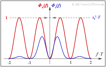
$$H_{\rm C}(f) = {1}/{2} \cdot \big [1 - K_{\rm C} \cdot {\rm e}^{-{\rm j}\hspace{0.03cm}\cdot \hspace{0.03cm} 2\pi\hspace{0.03cm}\cdot \hspace{0.03cm}f \hspace{0.03cm}\cdot \hspace{0.03cm} N_{\rm C}\hspace{0.03cm}\cdot \hspace{0.03cm}T} \big] ={1}/{2} \cdot \big [1 - K \cdot {\rm e}^{-{\rm j}\hspace{0.03cm}\cdot \hspace{0.03cm} \alpha} \big ]\hspace{0.05cm}.$$

This gives the power-spectral density $\rm (PSD)$ of the amplitude coefficients $(K$ and $\alpha$ are abbreviations according to the above equation$)$:

$$ {\it \Phi}_a(f) = | H_{\rm C}(f)|^2 = \frac{\big [1 - K \cos (\alpha) + {\rm j}\cdot K \sin (\alpha) \big ] \big [1 - K \cos (\alpha) - {\rm j}\cdot K \sin (\alpha) \big ] }{4} = \text{...} = {1}/{4} \cdot \big [2 - 2 \cdot K \cdot \cos (\alpha) \big ] $$

Power-spectral density of the AMI code

$$ \Rightarrow \hspace{0.3cm}{\it \Phi}_a(f) = | H_{\rm C}(f)|^2 = {1}/{2} \cdot \big [1 - K_{\rm C} \cdot \cos (2\pi f N_{\rm C} T)\big ] \hspace{0.4cm}\bullet\!\!-\!\!\!-\!\!\!-\!\!\circ \hspace{0.4cm} \varphi_a(\lambda \cdot T)\hspace{0.05cm}.$$

In particular, for the power-spectral density of the AMI code $(N_{\rm C} = K_{\rm C} = 1)$, we obtain:

$${\it \Phi}_a(f) = {1}/{2} \cdot \big [1 - \cos (2\pi f T)\big ] = \sin^2 (\pi f T)\hspace{0.05cm}.$$

The graph shows

the PSD ${\it \Phi}_a(f)$ of the amplitude coefficients (red curve), and

the PSD ${\it \Phi}_s(f)$ of the total transmitted signal (blue), valid for NRZ rectangular pulses.

One recognizes from this representation

that the AMI code has no DC component, since ${\it \Phi}_a(f = 0) = {\it \Phi}_s(f = 0) = 0$,

the power $P_{\rm S} = s_0^2/2$ of the AMI-coded transmitted signal $($integral over ${\it \Phi}_s(f)$ from $- \infty$ to $+\infty)$.

Notes:

The PSD of the HDB3 and B6ZS codes differs only slightly from that of the AMI code.

You can use the (German language) SWF applet "Signals, ACF, and PSD of pseudo-ternary codes" to clarify the topic discussed here.

Properties of the duobinary code

The duobinary code is defined by the code parameters $N_{\rm C} = 1$ and $K_{\rm C} = -1$. This gives the power-spectral density $\rm (PSD)$ of the amplitude coefficients and the PSD of the transmitted signal:

Power-spectral density of the duobinary code

$${\it \Phi}_a(f) ={1}/{2} \cdot \big [1 + \cos (2\pi f T)\big ] = \cos^2 (\pi f T)\hspace{0.05cm},$$

$$ {\it \Phi}_s(f) = s_0^2 \cdot T \cdot \cos^2 (\pi f T)\cdot {\rm si}^2 (\pi f T)= s_0^2 \cdot T \cdot {\rm si}^2 (2 \pi f T) \hspace{0.05cm}.$$

The graph shows the power-spectral density

of the amplitude coefficients ⇒ ${\it \Phi}_a(f)$ as a red curve,

of the total transmitted signal ⇒ ${\it \Phi}_s(f)$ as a blue curve.

In the second graph, the signals $q(t)$, $b(t)$ and $c(t) = s(t)$ are sketched. We refer here again to the (German language) SWF applet "Signals, ACF, and PSD of pseudo-ternary codes", which also clarifies the duobinary code.

Signals in duobinary coding

From these illustrations it is clear:

In the duobinary code, any number of symbols with same polarity ("+1" or "–1") can directly succeed each other ⇒ ${\it \Phi}_a(f = 0)=1$, ${\it \Phi}_s(f = 0) = 1/2 \cdot s_0^2 \cdot T$.

In contrast, for the duobinary code, the alternating sequence "... , +1, –1, +1, –1, +1, ..." does not occur, which is particularly disturbing with respect to intersymbol interference. Therefore, in the duobinary code: ${\it \Phi}_s(f = 1/(2T) = 0$.

The power-spectral density ${\it \Phi}_s(f)$ of the pseudo-ternary duobinary code is identical to the PSD with redundancy-free binary coding at half rate $($symbol duration $2T)$.

Error probability of the pseudo-ternary codes

The graph shows the "eye diagrams" (without noise) when using

Eye diagrams for AMI, duobinary and 4B3T coding

the AMI code (left),
the duobinary code (center),
the 4B3T code (right).

The same assumptions apply as on the section "Error probability of the 4B3T codes". In particular:

The system comparison is made under "peak constraint". Therefore, we use the rectangular basic transmission pulse.

The overall frequency response shows a raised cosine with best possible rolloff factor $r = 0.8$.

The noise power $\sigma_d^2$ is thus $12\%$ larger than with the matched filter (global optimum).

The results can be interpreted as follows:

One can see in the left graph that for the AMI code the horizontal lines at $+s_0$ and $-s_0$ are missing (DC signal freedom!), while for the duobinary code (middle graph) no transitions from $+s_0$ to $-s_0$ (and vice versa) are possible.

With the 4B3T code, you can see clearly more lines in the eye diagram than in the two left pictures. The redundancy-free ternary code would give almost the same result.

In the section quoted above, the symbol error probability of the 4B3T code for the parameter $10 \cdot \lg \hspace{0.05cm}(s_0^2 \cdot T/N_0) = 13 \ \rm dB$ was calculated as follows:

$${ \sigma_d}/{s_0} = 0.145 \hspace{0.3cm}\Rightarrow \hspace{0.3cm} p_{\rm S} = {4}/{3} \cdot {\rm Q} \left( \frac{s_0/2}{ \sigma_d} \right) \approx {4}/{3} \cdot {\rm Q} \left( 3.45 \right) = 3.7 \cdot 10^{-4} \hspace{0.05cm}.$$

Using a pseudo-ternary code results in a larger error probability because here the noise rms value is not reduced compared to redundancy-free binary coding:

$${ \sigma_d}/{s_0} = 0.167 \hspace{0.3cm}\Rightarrow \hspace{0.3cm} p_{\rm S} = {4}/{3} \cdot {\rm Q} \left( \frac{s_0/2}{ \sigma_d} \right) \approx {4}/{3} \cdot {\rm Q} \left( 3 \right) = 1.8 \cdot 10^{-3} \hspace{0.05cm}.$$

When the Nyquist condition is satisfied, the AMI and duobinary codes do not differ in terms of error probability despite completely different eye diagrams. But as will be shown in the section "Eye opening for the pseudo-ternary codes", the error behavior of these codes differs extremely whenever "intersymbol interference" plays a role.

Exercises for the chapter

Exercise 2.7: AMI Code

Exercise 2.7Z: Power-Spectral Density of Pseudo-Ternary Codes

Exercise 2.8: Code Comparison Binary, AMI and 4B3T

Symbolwise Coding with Pseudo-Ternary Codes

Contents

General description of the pseudo-multilevel codes

Properties of the AMI code

Power-spectral density of the AMI code

Properties of the duobinary code

Error probability of the pseudo-ternary codes

Exercises for the chapter