Difference between revisions of "Aufgaben:Exercise 1.5: Reconstruction of the Jakes Spectrum"
m (Text replacement - "===Solutions===" to "===Solution===") |
|||
| Line 84: | Line 84: | ||
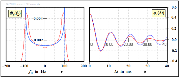
The graph shows the result of the approximation. The red curves were determined simulatively over $100\hspace{0.05cm}000$ samples. You can see: | The graph shows the result of the approximation. The red curves were determined simulatively over $100\hspace{0.05cm}000$ samples. You can see: | ||
| − | [[File:EN_Mob_A_1_5d.png|right|frame|Approximation of the Jakes spectrum and | + | [[File:EN_Mob_A_1_5d.png|right|frame|Approximation of the Jakes spectrum and the autocorrelation function]] |
* The Jakes PDS (left graph) can only be reproduced very inaccurately due to the vertical drop at $± f_{\rm D, \ max}$. | * The Jakes PDS (left graph) can only be reproduced very inaccurately due to the vertical drop at $± f_{\rm D, \ max}$. | ||
Revision as of 15:39, 12 February 2021
In a mobile radio system, the Doppler effect is also noticeable in the power density spectrum of the Doppler frequency $f_{\rm D}$.
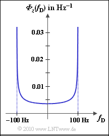
This results in the so-called Jakes spectrum, which is shown in the graph for the maximum Doppler frequency $f_{\rm D, \ max} = 100 \ \rm Hz$. ${\it \Phi}_z(f_{\rm D})$ has only portions within the range $± f_{\rm D, \ max}$, where
- $${\it \Phi}_z(f_{\rm D}) = \frac{2 \cdot \sigma^2}{\pi \cdot f_{\rm D, \hspace{0.1cm} max} \cdot \sqrt { 1 - (f_{\rm D}/f_{\rm D, \hspace{0.1cm} max})^2} } \hspace{0.05cm}.$$
What is expressed in the frequency domain by the power density spectrum $\rm (PDS)$ is described in the time domain by the autocorrelation function $\rm (ACF)$. The ACF is the ${\it \Phi}_z(f_{\rm D})$ by the inverse Fourier transform of the PDS.
With the Bessel function of the first kind and zero order $({\rm J}_0)$ you get
- $$\varphi_z ({\rm \Delta}t) = 2 \sigma^2 \cdot {\rm J_0}(2\pi \cdot f_{\rm D, \hspace{0.1cm} max} \cdot {\rm \Delta}t)\hspace{0.05cm}.$$
To take into account the Doppler effect and thus a relative movement between transmitter and receiver in a system simulation, two digital filters are inserted in the Rayleigh channel model, each with the frequency response $H_{\rm DF}(f_{\rm D})$.
The dimensioning of these filters is part of this task.
- We restrict ourselves here to the branch for generating the real part $x(t)$. The ratios derived here are also valid for the imaginary part $y(t)$.
- At the input of the left digital filter of the Rayleigh channel model , there is white Gaussian noise $n(t)$ with variance $\sigma^2 = 0.5$.
- The real component is then obtained from the following convolution
- $$x(t) = n(t) \star h_{\rm DF}(t) \hspace{0.05cm}.$$
Notes:
- This task belongs to the topic of Statistical bindings within the Rayleigh process.
- The digital filter is treated in detail in chapter Digital Filter of the book "Stochastic Signal Theory".
Questions
Solution
- $${\it \Phi}_x(f_{\rm D} = 0) = {\it \Phi}_y(f_{\rm D} = 0) = \frac{{\it \Phi}_z(f_{\rm D} = 0)}{2}= \frac{\sigma^2}{\pi \cdot f_{\rm D, \hspace{0.05cm} max}} = \frac{0.5}{\pi \cdot 100\,\,{\rm Hz}} \hspace{0.15cm} \underline{ = 1.59 \cdot 10^{-3}\,\,{\rm Hz^{-1}}} \hspace{0.05cm}.$$
(2) Solution 2 is correct:
- The input signal $n(t)$ has a white (constant) PDS ${\it \Phi}_n(f_{\rm D})$.
- The PDS at the output is then
- $${\it \Phi}_x(f_{\rm D}) = {\it \Phi}_n(f_{\rm D}) \cdot | H_{\rm DF}(f_{\rm D}|^2 \hspace{0.05cm}.$$
(3) Solution 3 is correct.
- Only if this condition is fulfilled, the signal $x(t)$ has the same variance $\sigma^2$ as the noise signal $n(t)$.
(4) No:
- The two conditions after subtasks (2) and (3) only refer to the magnitude of the digital filter.
- There is no constraint for the phase of the digital filter.
- This phase can be chosen arbitrarily. Usually it is chosen in such a way that a minimum phase network results.
- In this case, the impulse response $h_{\rm DF}(t)$ then has the lowest possible duration.
The graph shows the result of the approximation. The red curves were determined simulatively over $100\hspace{0.05cm}000$ samples. You can see:
- The Jakes PDS (left graph) can only be reproduced very inaccurately due to the vertical drop at $± f_{\rm D, \ max}$.
- For the time domain, this means that the ACF decreases much faster than the theory suggests.
- For small values of $\Delta t$, however, the approximation is very good (right graph).

