Difference between revisions of "Aufgaben:Exercise 4.6Z: Locality Curve for Phase Modulation"
| (9 intermediate revisions by 4 users not shown) | |||
| Line 1: | Line 1: | ||
| − | {{quiz-Header|Buchseite=Signal_Representation/ | + | {{quiz-Header|Buchseite=Signal_Representation/Equivalent Low-Pass Signal and its Spectral Function |
}} | }} | ||
| − | [[File:P_ID768__Sig_Z_4_6.png|right|frame| | + | [[File:P_ID768__Sig_Z_4_6.png|right|frame|A possible locality curve with phase modulation]] |
| − | + | We assume a source signal $q(t)$, which is considered normalised. | |
| − | * | + | *The maximum value of this signal is $q_{\rm max} = 1$ and the minimum signal value is $q_{\rm min} = -0.5$. |
| − | * | + | *Otherwise nothing is known about $q(t)$. |
| − | + | The modulated signal with phase modulation ⇒ "transmission signal" is: | |
:$$s(t) = s_0 \cdot {\cos} ( \omega_{\rm T}\hspace{0.05cm} t + \eta \cdot q(t)).$$ | :$$s(t) = s_0 \cdot {\cos} ( \omega_{\rm T}\hspace{0.05cm} t + \eta \cdot q(t)).$$ | ||
| − | + | Here $\eta$ denotes the so-called "modulation index". Let the constant envelope $s_0$ also be a normalise quantity, which is set to $s_0 = 2$ in the following (see diagram). | |
| − | + | If one replaces the cosine function with the complex exponential function, one arrives at the analytical signal | |
:$$s_{\rm +}(t) = s_0\cdot {\rm e}^{{\rm j}\hspace{0.05cm}\cdot \hspace{0.05cm}( | :$$s_{\rm +}(t) = s_0\cdot {\rm e}^{{\rm j}\hspace{0.05cm}\cdot \hspace{0.05cm}( | ||
\omega_{\rm T} \hspace{0.05cm}\cdot \hspace{0.05cm} t + \eta \hspace{0.05cm} \cdot \hspace{0.05cm} q(t)) }.$$ | \omega_{\rm T} \hspace{0.05cm}\cdot \hspace{0.05cm} t + \eta \hspace{0.05cm} \cdot \hspace{0.05cm} q(t)) }.$$ | ||
| − | + | From this, one can calculate the equivalent low-pass signal sketched in the graph as follows: | |
:$$s_{\rm TP}(t) = s_{\rm +}(t) \cdot {\rm e}^{-{\rm | :$$s_{\rm TP}(t) = s_{\rm +}(t) \cdot {\rm e}^{-{\rm | ||
j}\hspace{0.05cm} \cdot\hspace{0.05cm} \omega_{\rm T} \hspace{0.05cm}\cdot\hspace{0.05cm} t } = s_0\cdot | j}\hspace{0.05cm} \cdot\hspace{0.05cm} \omega_{\rm T} \hspace{0.05cm}\cdot\hspace{0.05cm} t } = s_0\cdot | ||
| Line 25: | Line 25: | ||
| + | ''Hints:'' | ||
| + | *This exercise belongs to the chapter [[Signal_Representation/Equivalent_Low-Pass_Signal_and_its_Spectral_Function|Equivalent Low-Pass Signal and its Spectral Function]]. | ||
| + | |||
| + | *You can check your solution with the interactive applet [[Applets:Physical_Signal_%26_Equivalent_Lowpass_Signal|Physical Signal & Equivalent Low-Pass Signal]] ⇒ "Locality Curve". | ||
| − | |||
| − | |||
| − | |||
| − | |||
| − | === | + | ===Questions=== |
<quiz display=simple> | <quiz display=simple> | ||
| − | { | + | {What is the magnitude function $a(t) = |s_{\rm TP}(t)|$? Which value is valid for $t = 0$? |
|type="{}"} | |type="{}"} | ||
$a(t = 0)\ = \ $ { 2 3% } | $a(t = 0)\ = \ $ { 2 3% } | ||
| − | { | + | {Between which extreme values $\phi_{\rm min}$ and $\phi_{\rm max}$ does the phase $\phi (t)$? |
|type="{}"} | |type="{}"} | ||
| − | $\phi_{\rm min}\ = \ $ { -93--87 } $\text{ | + | $\phi_{\rm min}\ = \ $ { -93--87 } $\text{deg}$ |
| − | $\phi_{\rm min}\ = \ $ { 180 3% } $\text{ | + | $\phi_{\rm min}\ = \ $ { 180 3% } $\text{deg}$ |
| − | { | + | {Determine the modulation index $\eta$ from the phase function $\phi (t)$. |
|type="{}"} | |type="{}"} | ||
$\eta\ = \ $ { 3.1415 3% } | $\eta\ = \ $ { 3.1415 3% } | ||
| − | { | + | {Which of the following statements are true? |
|type="[]"} | |type="[]"} | ||
| − | - | + | - From $q(t) = -0.5 = \text{const.}$ follows $s(t) = s_0 \cdot \cos (\omega_T \cdot t)$. |
| − | + | + | + With a rectangular signal $($with only two possible signal values $q(t)=\pm 0.5)$ the locality curve degenerates to two points. |
| − | + | + | + With the signal values $\pm 1$ $(q_{\rm min} = -0.5$ is then no longer valid$)$ the locality curve degenerates to one point: $s_{\rm TP}(t) = -s_0$. |
| Line 62: | Line 62: | ||
</quiz> | </quiz> | ||
| − | === | + | ===Solution=== |
{{ML-Kopf}} | {{ML-Kopf}} | ||
| − | '''(1)''' | + | '''(1)''' The locality curve is a circular arc with radius $2$. Therefore, the magnitude function is constant $\underline{a(t) = 2}$. |
| − | '''(2)''' | + | '''(2)''' From the graph it can be seen that the following numerical values apply: |
*$\phi_{\rm min} =- \pi /2 \; \Rightarrow \; \underline{-90^\circ}$, | *$\phi_{\rm min} =- \pi /2 \; \Rightarrow \; \underline{-90^\circ}$, | ||
*$\phi_{\rm max} = +\pi \; \Rightarrow \; \underline{+180^\circ}$. | *$\phi_{\rm max} = +\pi \; \Rightarrow \; \underline{+180^\circ}$. | ||
| Line 73: | Line 73: | ||
| − | '''(3)''' | + | '''(3)''' In general, the relation $s_{\rm TP}(t) = a(t) \cdot {\rm e}^{{\rm j}\hspace{0.05cm}\cdot \hspace{0.05cm} |
| − | \phi(t)}. | + | \phi(t)}$ applies here. A comparison with the given function yields: |
:$$\phi(t) = \eta \cdot q(t).$$ | :$$\phi(t) = \eta \cdot q(t).$$ | ||
| − | * | + | *The maximum phase value $\phi_{\rm max} = +\pi \; \Rightarrow \; {180^\circ}$ is obtained for the signal amplitude $q_{\rm max} = 1$. From this follows directly ${\eta = \pi} \; \underline{\approx 3.1415}$. |
| − | * | + | *This modulation index is confirmed by the values $\phi_{\rm min} = -\pi /2$ and $q_{\rm min} = -0.5$ . |
| − | [[File:P_ID769__Sig_Z_4_6_d_neu.png|right|frame| | + | [[File:P_ID769__Sig_Z_4_6_d_neu.png|right|frame|Locality curve (phase diagram) for a rectangular source signal]] |
| − | '''(4)''' | + | '''(4)''' <u>The second and third proposed solutions</u> are correct: |
| − | * | + | *If $q(t) = \text{const.} =-0.5$, the phase function is also constant: |
:$$\phi(t) = \eta \cdot q(t) = - {\pi}/{2}\hspace{0.3cm} | :$$\phi(t) = \eta \cdot q(t) = - {\pi}/{2}\hspace{0.3cm} | ||
\Rightarrow \hspace{0.3cm} s_{\rm TP}(t) = - {\rm j} \cdot s_0 = - 2{\rm j}.$$ | \Rightarrow \hspace{0.3cm} s_{\rm TP}(t) = - {\rm j} \cdot s_0 = - 2{\rm j}.$$ | ||
| − | * | + | *Thus, for the actual physical signal: |
:$$s(t) = s_0 \cdot {\cos} ( \omega_{\rm T}\hspace{0.05cm} t - | :$$s(t) = s_0 \cdot {\cos} ( \omega_{\rm T}\hspace{0.05cm} t - | ||
{\pi}/{2}) = 2 \cdot {\sin} ( \omega_{\rm T} \hspace{0.05cm} t ).$$ | {\pi}/{2}) = 2 \cdot {\sin} ( \omega_{\rm T} \hspace{0.05cm} t ).$$ | ||
| − | * | + | *In contrast, $q(t) = +0.5$ leads to $\phi (t) = \pi /2$ and to $s_{\rm TP}(t) = 2{\rm j}$. |
| − | * | + | *If $q(t)$ is a rectangular signal that alternates between $+0.5$ and $–0.5$ , then the locality curve consists of only two points on the imaginary axis, regardless of how long the intervals with $+0.5$ and $–0.5$ last. |
| − | * | + | *If, on the other hand, $q(t) = \pm 1$, then the possible phase values $+\pi$ and $-\pi$ result purely formally, but they are identical. |
| − | * | + | *The locality curve then consists of only one point: $s_{\rm TP}(t) = - s_0$ ⇒ the signal $s(t)$ is "minus-cosine" for all times $t$. |
| Line 98: | Line 98: | ||
__NOEDITSECTION__ | __NOEDITSECTION__ | ||
| − | [[Category: | + | [[Category:Signal Representation: Exercises|^4.3 Equivalent LP Signal and its Spectral Function^]] |
Latest revision as of 15:02, 24 May 2021
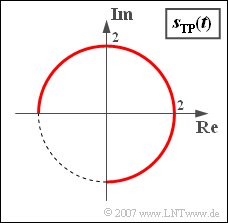
We assume a source signal $q(t)$, which is considered normalised.
- The maximum value of this signal is $q_{\rm max} = 1$ and the minimum signal value is $q_{\rm min} = -0.5$.
- Otherwise nothing is known about $q(t)$.
The modulated signal with phase modulation ⇒ "transmission signal" is:
- $$s(t) = s_0 \cdot {\cos} ( \omega_{\rm T}\hspace{0.05cm} t + \eta \cdot q(t)).$$
Here $\eta$ denotes the so-called "modulation index". Let the constant envelope $s_0$ also be a normalise quantity, which is set to $s_0 = 2$ in the following (see diagram).
If one replaces the cosine function with the complex exponential function, one arrives at the analytical signal
- $$s_{\rm +}(t) = s_0\cdot {\rm e}^{{\rm j}\hspace{0.05cm}\cdot \hspace{0.05cm}( \omega_{\rm T} \hspace{0.05cm}\cdot \hspace{0.05cm} t + \eta \hspace{0.05cm} \cdot \hspace{0.05cm} q(t)) }.$$
From this, one can calculate the equivalent low-pass signal sketched in the graph as follows:
- $$s_{\rm TP}(t) = s_{\rm +}(t) \cdot {\rm e}^{-{\rm j}\hspace{0.05cm} \cdot\hspace{0.05cm} \omega_{\rm T} \hspace{0.05cm}\cdot\hspace{0.05cm} t } = s_0\cdot {\rm e}^{{\rm j}\hspace{0.05cm}\cdot\hspace{0.05cm} \eta \hspace{0.05cm} \cdot \hspace{0.05cm} q(t) }.$$
Hints:
- This exercise belongs to the chapter Equivalent Low-Pass Signal and its Spectral Function.
- You can check your solution with the interactive applet Physical Signal & Equivalent Low-Pass Signal ⇒ "Locality Curve".
Questions
Solution
(2) From the graph it can be seen that the following numerical values apply:
- $\phi_{\rm min} =- \pi /2 \; \Rightarrow \; \underline{-90^\circ}$,
- $\phi_{\rm max} = +\pi \; \Rightarrow \; \underline{+180^\circ}$.
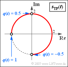
(3) In general, the relation $s_{\rm TP}(t) = a(t) \cdot {\rm e}^{{\rm j}\hspace{0.05cm}\cdot \hspace{0.05cm} \phi(t)}$ applies here. A comparison with the given function yields:
- $$\phi(t) = \eta \cdot q(t).$$
- The maximum phase value $\phi_{\rm max} = +\pi \; \Rightarrow \; {180^\circ}$ is obtained for the signal amplitude $q_{\rm max} = 1$. From this follows directly ${\eta = \pi} \; \underline{\approx 3.1415}$.
- This modulation index is confirmed by the values $\phi_{\rm min} = -\pi /2$ and $q_{\rm min} = -0.5$ .
(4) The second and third proposed solutions are correct:
- If $q(t) = \text{const.} =-0.5$, the phase function is also constant:
- $$\phi(t) = \eta \cdot q(t) = - {\pi}/{2}\hspace{0.3cm} \Rightarrow \hspace{0.3cm} s_{\rm TP}(t) = - {\rm j} \cdot s_0 = - 2{\rm j}.$$
- Thus, for the actual physical signal:
- $$s(t) = s_0 \cdot {\cos} ( \omega_{\rm T}\hspace{0.05cm} t - {\pi}/{2}) = 2 \cdot {\sin} ( \omega_{\rm T} \hspace{0.05cm} t ).$$
- In contrast, $q(t) = +0.5$ leads to $\phi (t) = \pi /2$ and to $s_{\rm TP}(t) = 2{\rm j}$.
- If $q(t)$ is a rectangular signal that alternates between $+0.5$ and $–0.5$ , then the locality curve consists of only two points on the imaginary axis, regardless of how long the intervals with $+0.5$ and $–0.5$ last.
- If, on the other hand, $q(t) = \pm 1$, then the possible phase values $+\pi$ and $-\pi$ result purely formally, but they are identical.
- The locality curve then consists of only one point: $s_{\rm TP}(t) = - s_0$ ⇒ the signal $s(t)$ is "minus-cosine" for all times $t$.

