Aufgaben:Exercise 1.2Z: Linear Distorting System

• Return to book

Deriving the distortions for square wave signals

The modulator, the channel, and the demodulator of a communication system can be represented by a single linear system with a frequency response of

$$ H(f) = {\rm si }( \pi \cdot f \cdot \Delta t)$$

The corresponding impulse response is rectangular, symmetrical about  $t = 0$  and has height  $1/Δt$  and (equivalent) duration  $Δt$ :

$$ h(t) = \left\{ \begin{array}{c} 1/\Delta t \\ 1/(2\Delta t) \\ 0 \\ \end{array} \right. \begin{array}{*{4}c} {\rm{for}} \\ {\rm{for}} \\ {\rm{for}} \\ \end{array}\begin{array}{*{20}c} {\left| \hspace{0.005cm} t\hspace{0.05cm} \right| < \Delta t/2,} \\ {\left| \hspace{0.005cm}t\hspace{0.05cm} \right| = \Delta t/2,} \\ {\left|\hspace{0.005cm} t \hspace{0.05cm} \right| > \Delta t/2.} \\ \end{array}$$

This is a slit low-pass filter, as discussed in the chapter  Some Low-Pass Functions in Systems Theory  in the book „Linear and Time Invariant Systems”.

The periodic square wave signal  $q(t)$  of period  $T_0$  is applied at the system input.  Thus, the duration of each rectangle and each gap is  $T_0/2$.  The height of the rectangles is  $2\ \rm V$.

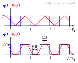
The signal  $v(t)$  at the system output is called the sink signal.  This is represented in the graph for two different parameter values with equivalent pulse duration (red waveforms):

• The signal  $v_1(t)$  results when the equivalent pulse duration of  $h(t)$  is exactly  $Δt_1$ .
• Accordingly, the signal  $v_2(t)$  is obtained with the equivalent pulse duration of  $Δt_2$.

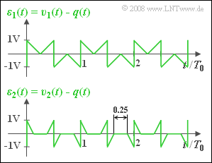
The change from the square wave signal  $q(t)$  to the triangular or trapezoidal sink signal  $v(t)$  is due to linear distortions and is captured by the error signal  $ε(t) = v(t) - q(t)$ .

Using the signal powers  $P_q$  and  $P_ε$  of  $q(t)$  and  $ε(t)$ , respectively, the sink SNR can be calculated:

$$\rho_{v} =P_{q}/{P_{\varepsilon }} \hspace{0.05cm}.$$

Hints:

• This exercise belongs to the chapter  Quality Criteria.  Particular reference is made to the page  Signal–to–noise (power) ratio and to the chapter  Linear Distortions im Buch "Linear and Time Invarian Systems".
• The powers  $P_q$  and  $P_ε$  are the root mean square values of the signals  $q(t)$  and  $ε(t)$  and can be determined for periodic signals with period duration  $T_0$  as follows:

$$P_{q} = \overline{q(t)^2} = \frac{1}{T_{\rm 0}} \cdot \int_{0}^{ T_{\rm 0}} {q(t)^2 }\hspace{0.1cm}{\rm d}t \hspace{0.05cm}, \hspace{0.5cm} P_{\varepsilon} = \overline{\varepsilon(t)^2} = \frac{1}{T_{\rm 0}} \cdot \int_{0}^{ T_{\rm 0}} {\varepsilon(t)^2 }\hspace{0.1cm}{\rm d}t \hspace{0.05cm}.$$

• Specifying the powers in  $\rm V^2$ , means that the signals refer to a resistance of  $R = 1\ \rm \Omega$ .

Questions

1

How long is the equivalent pulse duration  $Δt_1$  within the signal  $v_1(t)$, relative to the period   $T_0$?

$Δt_1/T_0 \ = \ $

2

What is the maximum value of the error signal  $ε_1(t) = v_1(t) - q(t)$?

$ε_\text{1, max} \ = \ $ $\ \rm V$

3

What is the "power"  $P_{ε1}$  of the error signal, i.e., the mean square deviation between  $v_1(t)$  and  $q(t)$?

$P_{ε1} \ = \ $ $\ \rm V^2$

4

Calculate the useful output  $P_q$  and the sink SNR  $ρ_{v1}$.

$P_q\ = \ $ $\ \rm V^2$

$ρ_{v1} \ = \ $

5

How long is the equivalent pulse duration  $Δt_2$  within the signal  $v_2(t)$, relative to the period  $T_0$?

$Δt_2/T_0 \ = \ $

6

Determine the error signal  $ε_2(t) = v_2(t) - q(t)$, the distortion power  $P_{ε2}$  and the sink SNR  $ρ_{v2}$.

$P_{ε2} \ = \ $ $\ \rm V^2$

$ρ_{v2} \ = \ $

7

Generalize your results for an arbitrary equivalent pulse duration  $Δt$.  What sink SNR  $ρ_{v3}$  results from  $Δt_3 = T_0/20$?

$ρ_{v3} \ = \ $

Solution

Solution

(1)   In general, Convolution of the periodic rectangular signal   $q(t)$  with the similarly rectangular impulse response  $h(t)$  only yields a triangular signal   $v(t)$, only if the rectangles involved have equal width. It follows:

$$\Delta t_1 = T_0 /2 \hspace{0.3cm}\Rightarrow \hspace{0.3cm} \Delta t_1 / T_0\hspace{0.15cm}\underline {= 0.5} \hspace{0.05cm}.$$

Fehlersignale bei den beiden betrachteten Empfangsfiltern unterschiedlicher Breite

(2)   The error signal   $ε_1(t)$  is shown in the adjacent graph.  It can be seen that  $ε_1(t)$ can assume all values in the range   $±1 \ \rm V$ :

$${\varepsilon}_\text{ 1, max} \hspace{0.15cm}\underline {= {1}\;{\rm V}} \hspace{0.05cm}.$$

(3)   It is sufficient to average over the time range from  $t = 0$  to  $t =T_0/4$, since all other subintervals contribute identically:

$$P_{\varepsilon{\rm 1}} = \frac{1}{T_{\rm 0}/4} \hspace{-0.05cm}\cdot \hspace{-0.05cm}\int_{0}^{ T_{\rm 0}/4} {\varepsilon_1(t)^2 }\hspace{0.1cm}{\rm d}t = \frac{1 \,{\rm V}^2}{T_{\rm 0}/4} \hspace{-0.05cm}\cdot \hspace{-0.05cm} \int_{0}^{ T_{\rm 0}/4} {\left( 1 - \frac{t}{T_{\rm 0}/4}\right)^2 }\hspace{0.1cm}{\rm d}t \hspace{0.05cm}.$$

• Substituting   $x = 4 · t/T_0$ , this can also be written as:

$$P_{\varepsilon{\rm 1}} = 1 \,{\rm V}^2 \hspace{-0.05cm}\cdot \hspace{-0.05cm} \int_{0}^{ 1} \hspace{-0.2cm}{\left( 1 - 2x + x^2\right)}\hspace{0.1cm}{\rm d}x \hspace{0.05cm}= 1 \,{\rm V}^2 \hspace{-0.05cm}\cdot \hspace{-0.05cm} \left( 1 - 1 + \frac{1}{3}\right)\hspace{0.15cm}\underline {= 0.333} \,{\rm V}^2\hspace{0.05cm}.$$

(4)   Averaging over one period of the squared source signal yields:

$$P_{q} = \frac{1}{T_0} \cdot \left[(2\,{\rm V})^2 \cdot \frac{T_0}{2}+(0\,{\rm V})^2 \cdot \frac{T_0}{2} \right]\hspace{0.15cm}\underline {= 2\,{\rm V^2}}\hspace{0.05cm}.$$

• The sink SNR is therefore

$$\rho_{v{\rm 1}} = \frac{P_{q}}{P_{\varepsilon {\rm 1}}} = \frac{2 \,{\rm V}^2}{0.333 \,{\rm V}^2}\hspace{0.15cm}\underline {= 6} \hspace{0.05cm}.$$

(5)   According to the sketch presented above, a rectangle of duration   $0.5 \cdot T_0$  now becomes a trapezoid of absolute duration  $0.75 · T_0$.

• Thus, according to the laws of convolution, it is obvious that the equivalent pulse duration must be  $Δt_2/T_0\hspace{0.15cm}\underline { = 0.25}$ .

(6)   The lower plot in the above graph shows that   $ε_2(t)$  is composed of four triangles within a period of   $T_0$  just like  $ε_1(t)$ , though they are only half as wide. 

• Thus, in half the time,   $ε_2(t) = 0$.

• Because of  $ε_\text{2, max} = ε_\text{1, max} = 1 \ \rm V$ , one obtains:

$$P_{\varepsilon{\rm 2}} ={P_{\varepsilon{\rm 1}}}/{2} \hspace{0.15cm}\underline {= 0.167} \,{\rm V}^2 \hspace{0.3cm}\Rightarrow \hspace{0.3cm} \rho_{v{\rm 2}} = {P_{q}}/{P_{\varepsilon {\rm 2}}}\hspace{0.15cm}\underline {= 12} \hspace{0.05cm}.$$

(7)   Für  $Δt = T_0/2$  wurde in der Teilaufgabe  (3)  die Verzerrungsleistung  $P_{ε1} = 1/3 \ \rm V^{ 2 }$  berechnet.

• In der Teilaufgabe  (6)  wurde gezeigt, dass bei  $Δt = T_0/4$  die Verzerrungsleistung  $P_{ε2}$  nur halb so groß ist.

• Anschaulich wurde erläutert, dass ein linearer Zusammenhang besteht.  Daraus folgen für  $Δt ≤ T_0/2$  die empirischen Gleichungen:

$$P_{\varepsilon} = \frac{2 \,{\rm V}^2}{3} \cdot \frac{\Delta t}{T_0} \hspace{0.3cm}\Rightarrow \hspace{0.3cm} \rho_{v} = \frac{P_{q}}{P_{\varepsilon }}= \frac{3}{\Delta t/T_0} \hspace{0.05cm}.$$

• Der Sonderfall  $Δt = T_0/20$  führt somit zu den Resultaten:

$$P_{\varepsilon{\rm 3}} = \frac{2 \,{\rm V}^2}{60} \hspace{0.3cm}\Rightarrow \hspace{0.3cm} \rho_{v{\rm 3}} = \frac{P_{q}}{P_{\varepsilon {\rm 3}}}\hspace{0.15cm}\underline {= 60} \hspace{0.05cm}.$$