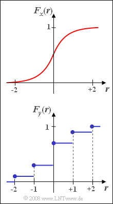
Difference between revisions of "Aufgaben:Exercise 3.2: CDF for Exercise 3.1"
| Line 20: | Line 20: | ||
Hints: | Hints: | ||
| − | *The | + | *The exercise belongs to the chapter [[Theory_of_Stochastic_Signals/Cumulative_Distribution_Function|cumulative distribution function]]. |
| − | |||
*Given the following equation: | *Given the following equation: | ||
:$$\int \cos^{\rm 2}( ax)\, {\rm d}x=\frac{x}{2}+\frac{1}{4 a}\cdot \sin(2 ax).$$ | :$$\int \cos^{\rm 2}( ax)\, {\rm d}x=\frac{x}{2}+\frac{1}{4 a}\cdot \sin(2 ax).$$ | ||
| − | The topic of this chapter is illustrated with examples in the (German language) learning video [[Zusammenhang_zwischen_WDF_und_VTF_(Lernvideo)|Zusammenhang zwischen WDF und VTF]] $\Rightarrow$ relationship between PDF and CDF. | + | *The topic of this chapter is illustrated with examples in the (German language) learning video [[Zusammenhang_zwischen_WDF_und_VTF_(Lernvideo)|Zusammenhang zwischen WDF und VTF]] $\Rightarrow$ relationship between PDF and CDF. |
Revision as of 21:59, 26 December 2021
The same conditions apply as for Exercise 3.1.
- The PDF of the continuous valued random variable is identically zero in the ranges $|x| > 2$ and in the range $-2 \le x \le +2$ holds:
- $$f_x(x)={1}/{2}\cdot \cos^2({\pi}/{4}\cdot x).$$
- Also, the discrete random variable $y$ is limited to the range $\pm 2$ Here, the following probabilities apply:
- $${\rm \Pr}(y=0)=0.4,$$
- $${\rm \Pr}(y=+1)={\rm \Pr}(y=-1)=0.2,$$
- $${\rm \Pr}(y=+2)={\rm \Pr}(y=-2)=0.1.$$
Hints:
- The exercise belongs to the chapter cumulative distribution function.
- Given the following equation:
- $$\int \cos^{\rm 2}( ax)\, {\rm d}x=\frac{x}{2}+\frac{1}{4 a}\cdot \sin(2 ax).$$
- The topic of this chapter is illustrated with examples in the (German language) learning video Zusammenhang zwischen WDF und VTF $\Rightarrow$ relationship between PDF and CDF.
Questions
Solution
(2) Only statements 2 and 3 are correct here:
- For a discrete random variable, the distribution function increases only weakly monotonically.
- That means: Except for unit steps, there are only horizontal sections of the CDF.
- Since at the unit step points the right-hand side limit value is valid, $F_y(-2) = 0.1$, i.e. not equal to zero.
(3) The CDF $F_x(r)$ is calculated as the integral from $-\infty$ to $r$ over the PDF $f_x(x)$.
Due to symmetry, herefore can be written in the range $0 \le r \le +2$ :
- $$F_{x} (r) =\frac{1}{2} + \int_{0}^{r} f_x(x)\;{\rm d}x = \frac{1}{2} + \int_{0}^{ r} {1}/{2}\cdot \cos^2 ({\pi}/{4}\cdot x)\;{\rm d}x.$$
In the same way as for the subtask (7) of Exercise 3.1, we thus obtain:
- $$F_{x} (r) =\frac{1}{2} + \frac{ r}{ 4} + \frac{1}{2 \pi} \cdot \sin({\pi}/{2}\cdot r),$$
- $$F_{x} (r=0) =\rm \frac{1}{2} + \rm \frac{1}{2 \pi} \cdot\rm sin(\rm 0)\hspace{0.15cm}{= 0.500},$$
- $$F_{x} (r=1) =\rm \frac{1}{2} + \frac{\rm 1}{\rm 4} + \rm \frac{1}{2 \pi}\cdot \rm sin({\pi}/{2})\hspace{0.15cm}\underline{=0.909},$$
- $$F_{x} (r=2) =\rm \frac{1}{2} + \frac{\rm1}{\rm 2} + \rm \frac{1}{2 \pi} \cdot \rm sin(\pi)\hspace{0.15cm}{= 1.000}.$$
(4) Because of the point symmetry around $r=0$ resp. $F_{x} (0) = 1/2$ and because of $\sin(-x) = -\sin(x)$ this formula holds in the whole domain, as the following control calculation shows:
- $$F_{x} (r=-2) =\rm \frac{1}{2} - \frac{\rm1}{\rm 2} - \rm \frac{1}{2 \pi} \cdot\rm sin(\pi)=0,$$
- $$F_{x} (r=-1) =\rm \frac{1}{2} - \frac{\rm1}{\rm 4} - \rm \frac{1}{2 \pi} \cdot\rm sin({\pi}/{2})\hspace{0.15cm}\underline{= 0.091}.$$
(5) For the probability that $x$ lies between $-1$ and $+1$ holds:
- $${\rm Pr}(|\hspace{0.05cm}x\hspace{0.05cm}|< 1)= F_{x}(+1) - F_{ x}(-1)= 0.909-0.091\hspace{0.15cm}\underline{= 0.818}.$$
- This result agrees exactly with the result of the subtask (7) of Exercise 3.1 üwhich was obtained by direct integration üover the WDF.
(6) The VTF of the discrete random sizeö&aerospace;e $y$ at the location $y =0$ is the sum of the probabilities of $-2$, $-1$ and $0$, so holds
- $$F_y(r = 0)\hspace{0.15cm}\underline{= 0.7}.$$
