Difference between revisions of "Theory of Stochastic Signals/Two-Dimensional Random Variables"
| Line 65: | Line 65: | ||
{{BlaueBox|TEXT= | {{BlaueBox|TEXT= | ||
$\text{Definition:}$ | $\text{Definition:}$ | ||
| − | The probability density function of the two-dimensional random variable at the location $(x_\mu, y_\mu)$ ⇒ '''joint PDF | + | The probability density function of the two-dimensional random variable at the location $(x_\mu, y_\mu)$ ⇒ '''joint PDF''' is an extension of the one-dimensional PDF $(∩$ denotes logical AND operation$)$: |
:$$f_{xy}(x_\mu, \hspace{0.1cm}y_\mu) = \lim_{\left.{\delta x\rightarrow 0 \atop {\delta y\rightarrow 0} }\right. }\frac{ {\rm Pr}\big [ (x_\mu - {\rm \Delta} x/{\rm 2} \le x \le x_\mu + {\rm \Delta} x/{\rm 2}) \cap (y_\mu - {\rm \Delta} y/{\rm 2} \le y \le y_\mu +{\rm \Delta}y/{\rm 2}) \big] }{ {\rm \delta} \ x\cdot{\rm \Delta} y}.$$ | :$$f_{xy}(x_\mu, \hspace{0.1cm}y_\mu) = \lim_{\left.{\delta x\rightarrow 0 \atop {\delta y\rightarrow 0} }\right. }\frac{ {\rm Pr}\big [ (x_\mu - {\rm \Delta} x/{\rm 2} \le x \le x_\mu + {\rm \Delta} x/{\rm 2}) \cap (y_\mu - {\rm \Delta} y/{\rm 2} \le y \le y_\mu +{\rm \Delta}y/{\rm 2}) \big] }{ {\rm \delta} \ x\cdot{\rm \Delta} y}.$$ | ||
$\rm Note$: | $\rm Note$: | ||
| Line 106: | Line 106: | ||
*For two-dimensional random variables, the PDF volume is always equal $1$.}} | *For two-dimensional random variables, the PDF volume is always equal $1$.}} | ||
| − | == | + | ==PDF and CDF for statistically independent components== |
<br> | <br> | ||
| − | + | For statistically independent components $x$ and $y$ the following holds for the joint probability according to the elementary laws of statistics if $x$ and $y$ are continuous in value: | |
:$${\rm Pr} \big[(x_{\rm 1}\le x \le x_{\rm 2}) \cap( y_{\rm 1}\le y\le y_{\rm 2})\big] ={\rm Pr} (x_{\rm 1}\le x \le x_{\rm 2}) \cdot {\rm Pr}(y_{\rm 1}\le y\le y_{\rm 2}) .$$ | :$${\rm Pr} \big[(x_{\rm 1}\le x \le x_{\rm 2}) \cap( y_{\rm 1}\le y\le y_{\rm 2})\big] ={\rm Pr} (x_{\rm 1}\le x \le x_{\rm 2}) \cdot {\rm Pr}(y_{\rm 1}\le y\le y_{\rm 2}) .$$ | ||
| − | + | For this, independent components can also be written: | |
:$${\rm Pr} \big[(x_{\rm 1}\le x \le x_{\rm 2}) \cap(y_{\rm 1}\le y\le y_{\rm 2})\big] =\int _{x_{\rm 1}}^{x_{\rm 2}}f_{x}(x) \,{\rm d}x\cdot \int_{y_{\rm 1}}^{y_{\rm 2}} f_{y}(y) \, {\rm d}y.$$ | :$${\rm Pr} \big[(x_{\rm 1}\le x \le x_{\rm 2}) \cap(y_{\rm 1}\le y\le y_{\rm 2})\big] =\int _{x_{\rm 1}}^{x_{\rm 2}}f_{x}(x) \,{\rm d}x\cdot \int_{y_{\rm 1}}^{y_{\rm 2}} f_{y}(y) \, {\rm d}y.$$ | ||
| − | {{BlaueBox|TEXT= | + | {{BlaueBox|TEXT= |
| − | $\text{Definition:}$ | + | $\text{Definition:}$ It follows that for '''statistical independence'''' the following condition must be satisfied with respect to the 2D–probability density function: |
:$$f_{xy}(x,y)=f_{x}(x) \cdot f_y(y) .$$}} | :$$f_{xy}(x,y)=f_{x}(x) \cdot f_y(y) .$$}} | ||
{{GraueBox|TEXT= | {{GraueBox|TEXT= | ||
| − | $\text{ | + | $\text{Example 2:}$ In the graph, the instantaneous values of a two-dimensional random variable are plotted as points in the $(x, y)$–plane. |
| − | * | + | *Ranges with many points, which accordingly appear dark, indicate large values of the 2D–WDF $f_{xy}(x, y)$. |
| − | * | + | *In contrast, the random variable $(x, y)$ has relatively few components in rather bright areas. |
| − | [[File:P_ID153__Sto_T_4_1_S4_nochmals_neu.png |frame| | + | [[File:P_ID153__Sto_T_4_1_S4_nochmals_neu.png |frame| Statistically independent components: $f_{xy}(x,y)$, $f_{x}(x)$ and $f_{y}(y)$]] |
| − | + | The graph can be interpreted as follows: | |
| − | * | + | *The marginal probability densities $f_{x}(x)$ and $f_{y}(y)$ already indicate that both $x$ and $y$ are Gaussian and zero mean, and that the random variable $x$ has a larger standard deviation than $y$ . |
| − | *$f_{x}(x)$ | + | *$f_{x}(x)$ and $f_{y}(y)$ however, do not provide information on whether or not statistical bindings exist for the random variable $(x, y)$ . |
| − | * | + | *However, using the 2D WDF $f_{xy}(x,y)$ one can see that there are no statistical bindings between the two components $x$ and $y$ here. |
| − | * | + | *With statistical independence, any cut through $f_{xy}(x, y)$ parallel to $y$-axis yields a function that is equal in shape to the edge–WDF $f_{y}(y)$. Similarly, all cuts parallel to $x$-axis are equal in shape to $f_{x}(x)$. |
| − | * | + | *This fact is equivalent to saying that in this example $f_{xy}(x, y)$ can be represented as the product of the two marginal probability densities: $f_{xy}(x,y)=f_{x}(x) \cdot f_y(y) .$}} |
| − | == | + | ==PDF and CDF for statistically dependent components== |
<br> | <br> | ||
| − | + | If there are statistical bindings between $x$ and $y$, then different cuts parallel to $x$– and $y$–axis, respectively, yield different, non-shape equivalent functions. In this case, of course, the joint–WDF cannot be described as a product of the two (one-dimensional) marginal probability densities either. | |
| − | [[File:P_ID156__Sto_T_4_1_S5_neu.png |right|frame| | + | [[File:P_ID156__Sto_T_4_1_S5_neu.png |right|frame|Statistically dependent components: $f_{xy}(x,y)$, $f_{x}(x)$, $f_{y}(y)$ ]] |
| − | {{GraueBox|TEXT= | + | {{GraueBox|TEXT= |
| − | $\text{ | + | $\text{Example 3:}$ The graph shows the instantaneous values of a two-dimensional random variable in the $(x, y)$–plane, where now, unlike $\text{Example 2}$ there are statistical bindings between $x$ and $y$ . |
| − | * | + | *The 2D–random variable takes all 2D–values with equal probability in the parallelogram drawn in blue. |
| − | * | + | *No values are possible outside the parallelogram. |
| − | + | One recognizes from this representation: | |
| − | * | + | *Integration over $f_{xy}(x, y)$ parallel to $x$–axis leads to the triangular marginal density $f_{y}(y)$, integration parallel to $y$–axis to the trapezoidal WDF $f_{x}(x)$. |
| − | * | + | *From the 2D-WDF $f_{xy}(x, y)$ it can already be guessed that for each $x$–value on statistical average a different $y$–value is to be expected. |
| − | * | + | *This means that here the components $x$ and $y$ are statistically dependent on each other. }} |
| − | == | + | ==Expected values of two-dimensional random variables== |
<br> | <br> | ||
| − | + | A special case of statistical dependence is ''correlation''. | |
| − | {{BlaueBox|TEXT= | + | {{BlaueBox|TEXT= |
| − | $\text{Definition:}$ | + | $\text{Definition:}$ Under '''correlation''' one understands a ''linear dependence'' between the individual components $x$ and $y$. |
| − | * | + | *Correlated random variables are thus always also statistically dependent. |
| − | * | + | *But not every statistical dependence implies correlation at the same time}}. |
| − | + | To quantitatively capture correlation, one uses various expected values of the 2D random variable $(x, y)$. | |
| − | + | These are defined analogously to the one-dimensional case. | |
| − | * | + | *according to [[Theory_of_Stochastic_Signals/Moments_of_a_Discrete_Random_Variable|Chapter 2]] (for discrete value random variables). |
| − | *bzw. [[Theory_of_Stochastic_Signals/ | + | *bzw. [[Theory_of_Stochastic_Signals/Expected_Values_and_Moments|Chapter 3]] (for continuous value random variables): |
{{BlaueBox|TEXT= | {{BlaueBox|TEXT= | ||
| − | $\text{Definition:}$ | + | $\text{Definition:}$ For the (non-centered) '''moments''' the relation holds: |
:$$m_{kl}={\rm E}\big[x^k\cdot y^l\big]=\int_{-\infty}^{+\infty}\hspace{0.2cm}\int_{-\infty}^{+\infty} x\hspace{0.05cm}^{k} \cdot y\hspace{0.05cm}^{l} \cdot f_{xy}(x,y) \, {\rm d}x\, {\rm d}y.$$ | :$$m_{kl}={\rm E}\big[x^k\cdot y^l\big]=\int_{-\infty}^{+\infty}\hspace{0.2cm}\int_{-\infty}^{+\infty} x\hspace{0.05cm}^{k} \cdot y\hspace{0.05cm}^{l} \cdot f_{xy}(x,y) \, {\rm d}x\, {\rm d}y.$$ | ||
| − | + | Thus, the two linear means are $m_x = m_{10}$ and $m_y = m_{01}.$ }} | |
{{BlaueBox|TEXT= | {{BlaueBox|TEXT= | ||
| − | $\text{ | + | $\text{definition:}$ The $m_x$ and $m_y$ related '''central moments''' respectively are: |
:$$\mu_{kl} = {\rm E}\big[(x-m_{x})\hspace{0.05cm}^k \cdot (y-m_{y})\hspace{0.05cm}^l\big] .$$ | :$$\mu_{kl} = {\rm E}\big[(x-m_{x})\hspace{0.05cm}^k \cdot (y-m_{y})\hspace{0.05cm}^l\big] .$$ | ||
| − | In | + | In this general definition equation, the variances $σ_x^2$ and $σ_y^2$ of the two individual components are included by $\mu_{20}$ and $\mu_{02}$ respectively. }} |
| − | {{BlaueBox|TEXT= | + | {{BlaueBox|TEXT= |
| − | $\text{Definition:}$ | + | $\text{Definition:}$ Of particular importance is the '''covariance''' $(k = l = 1)$, which is a measure of the ''linear statistical dependence'' between the random variables $x$ and $y$ : |
| − | :$$\mu_{11} = {\rm E}\big[(x-m_{x})\cdot(y-m_{y})\big] = \int_{-\infty}^{+\infty} \int_{-\infty}^{+\infty} (x-m_{x}) \cdot (y-m_{y})\cdot f_{xy}(x,y) \,{\rm d}x \, | + | :$$\mu_{11} = {\rm E}\big[(x-m_{x})\cdot(y-m_{y})\big] = \int_{-\infty}^{+\infty} \int_{-\infty}^{+\infty} (x-m_{x}) \cdot (y-m_{y})\cdot f_{xy}(x,y) \,{\rm d}x \, {\rm d}y .$$ |
| − | + | In the following, we also denote the covariance $\mu_{11}$ in part by $\mu_{xy}$, if the covariance refers to the random variables $x$ and $y$ }} | |
| − | + | Notes: | |
| − | * | + | *The covariance $\mu_{11}=\mu_{xy}$ is related to the non-centered moment $m_{11} = m_{xy} = {\rm E}\big[x \cdot y\big]$ as follows: |
:$$\mu_{xy} = m_{xy} -m_{x }\cdot m_{y}.$$ | :$$\mu_{xy} = m_{xy} -m_{x }\cdot m_{y}.$$ | ||
| − | * | + | *This equation is enormously advantageous for numerical evaluations, since $m_{xy}$, $m_x$ and $m_y$ can be found from the sequences $〈x_v〉$ and $〈y_v〉$ in a single run. |
| − | * | + | *On the other hand, if one were to calculate the covariance $\mu_{xy}$ according to the above definition equation, one would have to find the mean values $m_x$ and $m_y$ in a first run and could then only calculate the expected value ${\rm E}\big[(x - m_x) \cdot (y - m_y)\big]$ in a second run. |
| − | [[File:P_ID628__Sto_T_4_1_S6Neu.png |right|frame| | + | [[File:P_ID628__Sto_T_4_1_S6Neu.png |right|frame| Example 2D expected values]] |
{{GraueBox|TEXT= | {{GraueBox|TEXT= | ||
| − | $\text{ | + | $\text{Example 4:}$ In the first two rows of the table, the respective first elements of two random sequences $〈x_ν〉$ and $〈y_ν〉$ are entered. In the last row, the respective products $x_ν - y_ν$ are given. |
| − | * | + | *By averaging over the ten sequence elements in each case, one obtains |
:$$m_x =0.5,\ \ m_y = 1, \ \ m_{xy} = 0.69.$$ | :$$m_x =0.5,\ \ m_y = 1, \ \ m_{xy} = 0.69.$$ | ||
| − | * | + | *This directly results in the value for the covariance: |
:$$\mu_{xy} = 0.69 - 0.5 · 1 = 0.19.$$ | :$$\mu_{xy} = 0.69 - 0.5 · 1 = 0.19.$$ | ||
<br clear=all> | <br clear=all> | ||
| − | + | Without knowledge of the equation $\mu_{xy} = m_{xy} - m_x\cdot m_y$ one would have had to first determine the mean values $m_x$ and $m_y$ in the first run,<br>in order to then determine the covariance $\mu_{xy}$ as the expected value of the product of the mean-free variables in a second run.}} | |
==Korrelationskoeffizient== | ==Korrelationskoeffizient== | ||
Revision as of 20:15, 13 January 2022
Contents
- 1 # OVERVIEW OF THE FOURTH MAIN CHAPTER #
- 2 Properties and examples
- 3 Joint PDF
- 4 Two-dimensional CDF
- 5 PDF and CDF for statistically independent components
- 6 PDF and CDF for statistically dependent components
- 7 Expected values of two-dimensional random variables
- 8 Korrelationskoeffizient
- 9 Korrelationsgerade
- 10 Aufgaben zum Kapitel
# OVERVIEW OF THE FOURTH MAIN CHAPTER #
Now random variables with statistical bindings are treated and illustrated by typical examples. After the general description of two-dimensional random variables, we turn to the autocorrelation function (ACF), the cross correlation function (CCF) and the associated spectral functions (PSD, CPSD) .
Specifically, it covers:
- the statistical description of 2D random variables using the (joint) PDF,
- the difference between statistical dependence and correlation, ???
- the classification features stationarity and ergodicity of stochastic processes,
- the definitions of autocorrelation function (ACF) and power spectral density (PSD),
- the definitions of cross correlation function and cross power spectral density, and
- the numerical determination of all these quantities in the two- and multi-dimensional cases.
For more information on Two-Dimensional Random Variables, as well as tasks, simulations, and programming exercises, see
- Chapter 5: Two-dimensional random variables (program "zwd")
- Chapter 9: Stochastic Processes (program "sto")
of the practical course "Simulation Methods in Communications Engineering". This (former) LNT course at the TU Munich is based on
- the teaching software package LNTsim ⇒ Link refers to the German ZIP–version of the program,
- Internship Guide – Part A ⇒ Link refers to the German PDF–version with chapter 5: pages 81-97,
- the Internship Guide – Part B ⇒ Link refers to the German PDF–version with chapter 9: pages 207-228.
Properties and examples
As a transition to the correlation functions we now consider two random variables $x$ and $y$, between which statistical bindings(???) exist. Each of the two random variables can be described on its own with the introduced characteristic quantities
- corresponding to the second main chapter ⇒ Discrete Random Variables
- but the third main chapter ⇒ Continuous Random Variables.
$\text{Definition:}$ To describe the correlations between two variables $x$ and $y$ it is convenient to combine the two components into one two-dimensional random variable $(x, y)$ }.
- The individual components can be signals such as the real– and imaginary parts of a phase modulated signal.
- But there are a variety of 2D–random variables in other domains as well, as the following example will show
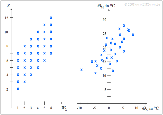
$\text{Example 1:}$ The left diagram is from the random experiment "Throwing two dice". Plotted to the right is the number of the first die $(W_1)$, plotted to the top is the sum $S$ of both dice. The two components here are each discrete random variables between which there are statistical dependencies(???):
- If $W_1 = 1$, then $S$ can only take values between $2$ and $7$ and each with equal probability.
- In contrast, for $W_1 = 6$ all values between $7$ and $12$ are possible, also with equal probability.
In the right graph, the maximum temperatures of the $31$ days in May 2002 of Munich (to the top) and the Zugspitze (to the right) are contrasted. Both random variables are continuous in value:
- although the measurement points are about $\text{100 km}$ apart, and on the Zugspitze, due to the different altitudes $($nearly $3000$ versus $520$ meters$)$ is on average about $20$ degrees colder than in Munich, one recognizes nevertheless a certain statistical dependence between the two random variables ${\it Θ}_{\rm M}$ and ${\it Θ}_{\rm Z}$.
- If it is warm in Munich, then pleasant temperatures are also more likely to be expected on the Zugspitze. However, the relationship is not deterministic: The coldest day in May 2002 was a different day in Munich than the coldest day on the Zugspitze.
Joint PDF
We restrict ourselves here mostly to continuous random variables. However, sometimes the peculiarities of two-dimensional discrete random variables are discussed in more detail. Most of the characteristics previously defined for one-dimensional random variables can be easily extended to two-dimensional variables.
$\text{Definition:}$ The probability density function of the two-dimensional random variable at the location $(x_\mu, y_\mu)$ ⇒ joint PDF is an extension of the one-dimensional PDF $(∩$ denotes logical AND operation$)$:
- $$f_{xy}(x_\mu, \hspace{0.1cm}y_\mu) = \lim_{\left.{\delta x\rightarrow 0 \atop {\delta y\rightarrow 0} }\right. }\frac{ {\rm Pr}\big [ (x_\mu - {\rm \Delta} x/{\rm 2} \le x \le x_\mu + {\rm \Delta} x/{\rm 2}) \cap (y_\mu - {\rm \Delta} y/{\rm 2} \le y \le y_\mu +{\rm \Delta}y/{\rm 2}) \big] }{ {\rm \delta} \ x\cdot{\rm \Delta} y}.$$
$\rm Note$:
- If the 2D–random variable is discrete, the definition must be slightly modified:
- For the lower range limits in each case, the "≤" sign must then be replaced by the "<" sign according to the page CDF for discrete random variables
.
Using this (joint) WDF $f_{xy}(x, y)$ statistical dependencies within the two-dimensional random variable $(x, y)$ are also fully captured in contrast to the two one-dimensional density functions ⇒ marginal probability density functions:
- $$f_{x}(x) = \int _{-\infty}^{+\infty} f_{xy}(x,y) \,\,{\rm d}y ,$$
- $$f_{y}(y) = \int_{-\infty}^{+\infty} f_{xy}(x,y) \,\,{\rm d}x .$$
These two marginal density functions $f_x(x)$ and $f_y(y)$
- provide only statistical information about the individual components $x$ and $y$, respectively,
- but not about the bindings between them.
Two-dimensional CDF
$\text{Definition:}$ The 2D distribution function like the 2D WDF, is merely a useful extension of the one-dimensional distribution function (CDF):
- $$F_{xy}(r_{x},r_{y}) = {\rm Pr}\big [(x \le r_{x}) \cap (y \le r_{y}) \big ] .$$
The following similarities and differences between the 1D CDF and the 2D CDF emerge:
- The functional relationship between two-dimensional PDF and two-dimensional VTF is given by integration as in the one-dimensional case, but now in two dimensions. For continuous random variables:
- $$F_{xy}(r_{x},r_{y})=\int_{-\infty}^{r_{y}} \int_{-\infty}^{r_{x}} f_{xy}(x,y) \,\,{\rm d}x \,\, {\rm d}y .$$
- Inversely, the probability density function can be given from the distribution function by partial differentiation to $r_{x}$ and $r_{y}$ :
- $$f_{xy}(x,y)=\frac{{\rm d}^{\rm 2} F_{xy}(r_{x},r_{y})}{{\rm d} r_{x} \,\, {\rm d} r_{y}}\Bigg|_{\left.{r_{x}=x \atop {r_{y}=y}}\right.}.$$
- Relative to the distribution function $F_{xy}(r_{x}, r_{y})$ the following limits apply:
- $$F_{xy}(-\infty,-\infty) = 0,$$
- $$F_{xy}(r_{\rm x},+\infty)=F_{x}(r_{x} ),$$
- $$F_{xy}(+\infty,r_{y})=F_{y}(r_{y} ) ,$$
- $$F_{xy} (+\infty,+\infty) = 1.$$
- In the limiting case $($infinitely large $r_{x}$ and $r_{y})$ Thus, for the 2D VTF, the value $1$. From this, we obtain the normalization condition for the 2D WDF:
- $$\int_{-\infty}^{+\infty} \int_{-\infty}^{+\infty} f_{xy}(x,y) \,\,{\rm d}x \,\,{\rm d}y=1 . $$
$\text{Conclusion:}$ Note the significant difference between one-dimensional and two-dimensional random variables:
- For one-dimensional random variables, the area under the PDF always yields the value $1$.
- For two-dimensional random variables, the PDF volume is always equal $1$.
PDF and CDF for statistically independent components
For statistically independent components $x$ and $y$ the following holds for the joint probability according to the elementary laws of statistics if $x$ and $y$ are continuous in value:
- $${\rm Pr} \big[(x_{\rm 1}\le x \le x_{\rm 2}) \cap( y_{\rm 1}\le y\le y_{\rm 2})\big] ={\rm Pr} (x_{\rm 1}\le x \le x_{\rm 2}) \cdot {\rm Pr}(y_{\rm 1}\le y\le y_{\rm 2}) .$$
For this, independent components can also be written:
- $${\rm Pr} \big[(x_{\rm 1}\le x \le x_{\rm 2}) \cap(y_{\rm 1}\le y\le y_{\rm 2})\big] =\int _{x_{\rm 1}}^{x_{\rm 2}}f_{x}(x) \,{\rm d}x\cdot \int_{y_{\rm 1}}^{y_{\rm 2}} f_{y}(y) \, {\rm d}y.$$
$\text{Definition:}$ It follows that for statistical independence' the following condition must be satisfied with respect to the 2D–probability density function:
- $$f_{xy}(x,y)=f_{x}(x) \cdot f_y(y) .$$
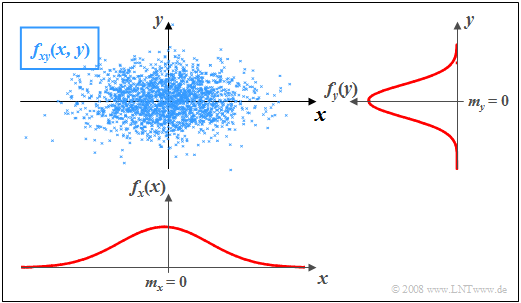
$\text{Example 2:}$ In the graph, the instantaneous values of a two-dimensional random variable are plotted as points in the $(x, y)$–plane.
- Ranges with many points, which accordingly appear dark, indicate large values of the 2D–WDF $f_{xy}(x, y)$.
- In contrast, the random variable $(x, y)$ has relatively few components in rather bright areas.
The graph can be interpreted as follows:
- The marginal probability densities $f_{x}(x)$ and $f_{y}(y)$ already indicate that both $x$ and $y$ are Gaussian and zero mean, and that the random variable $x$ has a larger standard deviation than $y$ .
- $f_{x}(x)$ and $f_{y}(y)$ however, do not provide information on whether or not statistical bindings exist for the random variable $(x, y)$ .
- However, using the 2D WDF $f_{xy}(x,y)$ one can see that there are no statistical bindings between the two components $x$ and $y$ here.
- With statistical independence, any cut through $f_{xy}(x, y)$ parallel to $y$-axis yields a function that is equal in shape to the edge–WDF $f_{y}(y)$. Similarly, all cuts parallel to $x$-axis are equal in shape to $f_{x}(x)$.
- This fact is equivalent to saying that in this example $f_{xy}(x, y)$ can be represented as the product of the two marginal probability densities: $f_{xy}(x,y)=f_{x}(x) \cdot f_y(y) .$
PDF and CDF for statistically dependent components
If there are statistical bindings between $x$ and $y$, then different cuts parallel to $x$– and $y$–axis, respectively, yield different, non-shape equivalent functions. In this case, of course, the joint–WDF cannot be described as a product of the two (one-dimensional) marginal probability densities either.
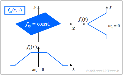
$\text{Example 3:}$ The graph shows the instantaneous values of a two-dimensional random variable in the $(x, y)$–plane, where now, unlike $\text{Example 2}$ there are statistical bindings between $x$ and $y$ .
- The 2D–random variable takes all 2D–values with equal probability in the parallelogram drawn in blue.
- No values are possible outside the parallelogram.
One recognizes from this representation:
- Integration over $f_{xy}(x, y)$ parallel to $x$–axis leads to the triangular marginal density $f_{y}(y)$, integration parallel to $y$–axis to the trapezoidal WDF $f_{x}(x)$.
- From the 2D-WDF $f_{xy}(x, y)$ it can already be guessed that for each $x$–value on statistical average a different $y$–value is to be expected.
- This means that here the components $x$ and $y$ are statistically dependent on each other.
Expected values of two-dimensional random variables
A special case of statistical dependence is correlation.
$\text{Definition:}$ Under correlation one understands a linear dependence between the individual components $x$ and $y$.
- Correlated random variables are thus always also statistically dependent.
- But not every statistical dependence implies correlation at the same time
.
To quantitatively capture correlation, one uses various expected values of the 2D random variable $(x, y)$.
These are defined analogously to the one-dimensional case.
- according to Chapter 2 (for discrete value random variables).
- bzw. Chapter 3 (for continuous value random variables):
$\text{Definition:}$ For the (non-centered) moments the relation holds:
- $$m_{kl}={\rm E}\big[x^k\cdot y^l\big]=\int_{-\infty}^{+\infty}\hspace{0.2cm}\int_{-\infty}^{+\infty} x\hspace{0.05cm}^{k} \cdot y\hspace{0.05cm}^{l} \cdot f_{xy}(x,y) \, {\rm d}x\, {\rm d}y.$$
Thus, the two linear means are $m_x = m_{10}$ and $m_y = m_{01}.$
$\text{definition:}$ The $m_x$ and $m_y$ related central moments respectively are:
- $$\mu_{kl} = {\rm E}\big[(x-m_{x})\hspace{0.05cm}^k \cdot (y-m_{y})\hspace{0.05cm}^l\big] .$$
In this general definition equation, the variances $σ_x^2$ and $σ_y^2$ of the two individual components are included by $\mu_{20}$ and $\mu_{02}$ respectively.
$\text{Definition:}$ Of particular importance is the covariance $(k = l = 1)$, which is a measure of the linear statistical dependence between the random variables $x$ and $y$ :
- $$\mu_{11} = {\rm E}\big[(x-m_{x})\cdot(y-m_{y})\big] = \int_{-\infty}^{+\infty} \int_{-\infty}^{+\infty} (x-m_{x}) \cdot (y-m_{y})\cdot f_{xy}(x,y) \,{\rm d}x \, {\rm d}y .$$
In the following, we also denote the covariance $\mu_{11}$ in part by $\mu_{xy}$, if the covariance refers to the random variables $x$ and $y$
Notes:
- The covariance $\mu_{11}=\mu_{xy}$ is related to the non-centered moment $m_{11} = m_{xy} = {\rm E}\big[x \cdot y\big]$ as follows:
- $$\mu_{xy} = m_{xy} -m_{x }\cdot m_{y}.$$
- This equation is enormously advantageous for numerical evaluations, since $m_{xy}$, $m_x$ and $m_y$ can be found from the sequences $〈x_v〉$ and $〈y_v〉$ in a single run.
- On the other hand, if one were to calculate the covariance $\mu_{xy}$ according to the above definition equation, one would have to find the mean values $m_x$ and $m_y$ in a first run and could then only calculate the expected value ${\rm E}\big[(x - m_x) \cdot (y - m_y)\big]$ in a second run.
$\text{Example 4:}$ In the first two rows of the table, the respective first elements of two random sequences $〈x_ν〉$ and $〈y_ν〉$ are entered. In the last row, the respective products $x_ν - y_ν$ are given.
- By averaging over the ten sequence elements in each case, one obtains
- $$m_x =0.5,\ \ m_y = 1, \ \ m_{xy} = 0.69.$$
- This directly results in the value for the covariance:
- $$\mu_{xy} = 0.69 - 0.5 · 1 = 0.19.$$
Without knowledge of the equation $\mu_{xy} = m_{xy} - m_x\cdot m_y$ one would have had to first determine the mean values $m_x$ and $m_y$ in the first run,
in order to then determine the covariance $\mu_{xy}$ as the expected value of the product of the mean-free variables in a second run.
Korrelationskoeffizient
Bei statististischer Unabhängigkeit der beiden Komponenten $x$ und $y$ ist die Kovarianz $\mu_{xy} \equiv 0$. Dieser Fall wurde bereits im $\text{Beispiel 2}$ auf der Seite WDF und VTF bei statistisch unabhängigen Komponenten betrachtet.
- Das Ergebnis $\mu_{xy} = 0$ ist aber auch bei statistisch abhängigen Komponenten $x$ und $y$ möglich, nämlich dann, wenn diese unkorreliert, also linear unabhängig sind.
- Die statistische Abhängigkeit ist dann nicht von erster, sondern von höherer Ordnung, zum Beispiel entsprechend der Gleichung $y=x^2.$
Man spricht von vollständiger Korrelation, wenn die (deterministische) Abhängigkeit zwischen $x$ und $y$ durch die Gleichung $y = K · x$ ausgedrückt wird. Dann ergibt sich für die Kovarianz:
- $\mu_{xy} = σ_x · σ_y$ bei positivem Wert von $K$,
- $\mu_{xy} = - σ_x · σ_y$ bei negativem $K$–Wert.
Deshalb verwendet man häufig als Beschreibungsgröße anstelle der Kovarianz den so genannten Korrelationskoeffizienten.
$\text{Definition:}$ Der Korrelationskoeffizient ist der Quotient aus der Kovarianz $\mu_{xy}$ und dem Produkt der Effektivwerte $σ_x$ und $σ_y$ der beiden Komponenten:
- $$\rho_{xy}=\frac{\mu_{xy} }{\sigma_x \cdot \sigma_y}.$$
Der Korrelationskoeffizient $\rho_{xy}$ weist folgende Eigenschaften auf:
- Aufgrund der Normierung gilt stets $-1 \le ρ_{xy} ≤ +1$.
- Sind die beiden Zufallsgrößen $x$ und $y$ unkorreliert, so ist $ρ_{xy} = 0$.
- Bei strenger linearer Abhängigkeit zwischen $x$ und $y$ ist $ρ_{xy}= ±1$ ⇒ vollständige Korrelation.
- Ein positiver Korrelationskoeffizient bedeutet, dass bei größerem $x$–Wert im statistischen Mittel auch $y$ größer ist als bei kleinerem $x$.
- Dagegen drückt ein negativer Korrelationskoeffizient aus, dass $y$ mit steigendem $x$ im Mittel kleiner wird.
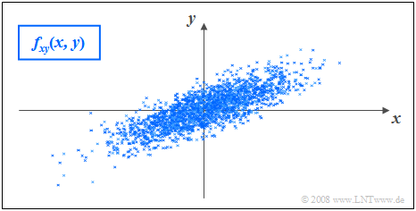
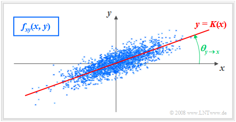
$\text{Beispiel 5:}$ Es gelten folgende Voraussetzungen:
- Die betrachteten Komponenten $x$ und $y$ besitzen jeweils eine gaußförmige WDF.
- Die beiden Streuungen sind unterschiedlich $(σ_y < σ_x)$.
- Der Korrelationskoeffizient beträgt $ρ_{xy} = 0.8$.
Im Unterschied zum Beispiel 2 mit statistisch unabhängigen Komponenten ⇒ $ρ_{xy} = 0$ $($trotz $σ_y < σ_x)$ erkennt man, dass hier bei größerem $x$–Wert im statistischen Mittel auch $y$ größer ist als bei kleinerem $x$.
Korrelationsgerade
$\text{Definition:}$ Als Korrelationsgerade bezeichnet man die Gerade $y = K(x)$ in der $(x, y)$–Ebene durch den „Mittelpunkt” $(m_x, m_y)$. Manchmal wird diese Gerade auch Regressionsgerade genannt.
Die Korrelationsgerade besitzt folgende Eigenschaften:
- Die mittlere quadratische Abweichung von dieser Geraden – in $y$–Richtung betrachtet und über alle $N$ Punkte gemittelt – ist minimal:
- $$\overline{\varepsilon_y^{\rm 2} }=\frac{\rm 1}{N} \cdot \sum_{\nu=\rm 1}^{N}\; \;\big [y_\nu - K(x_{\nu})\big ]^{\rm 2}={\rm Minimum}.$$
- Die Korrelationsgerade kann als eine Art „statistische Symmetrieachse“ interpretiert werden. Die Geradengleichung lautet:
- $$y=K(x)=\frac{\sigma_y}{\sigma_x}\cdot\rho_{xy}\cdot(x - m_x)+m_y.$$
Der Winkel, den die Korrelationsgerade zur $x$–Achse einnimmt, beträgt:
- $$\theta_{y\hspace{0.05cm}\rightarrow \hspace{0.05cm}x}={\rm arctan}\ (\frac{\sigma_{y} }{\sigma_{x} }\cdot \rho_{xy}).$$
Durch diese Nomenklatur soll deutlich gemacht werden, dass es sich hier um die Regression von $y$ auf $x$ handelt.
- Die Regression in Gegenrichtung – also von $x$ auf $y$ – bedeutet dagegen die Minimierung der mittleren quadratischen Abweichung in $x$–Richtung.
- Das interaktive Applet Korrelationskoeffizient und Regressionsgerade verdeutlicht, dass sich im Allgemeinen $($falls $σ_y \ne σ_x)$ für die Regression von $x$ auf $y$ ein anderer Winkel und damit auch eine andere Regressionsgerade ergeben wird:
- $$\theta_{x\hspace{0.05cm}\rightarrow \hspace{0.05cm} y}={\rm arctan}\ (\frac{\sigma_{x}}{\sigma_{y}}\cdot \rho_{xy}).$$
Aufgaben zum Kapitel
Aufgabe 4.1: Dreieckiges (x, y)-Gebiet
Aufgabe 4.1Z: Verabredung zum Frühstück
Aufgabe 4.1: Wieder Dreieckgebiet
Aufgabe 4.2Z: Korrelation zwischen $x$ und $e^x$
Aufgabe 4.3: Algebraische und Modulo-Summe
Aufgabe 4.3Z: Diracförmige 2D-WDF
