Difference between revisions of "Digital Signal Transmission/Optimal Receiver Strategies"
| Line 177: | Line 177: | ||
*If the input signal does not have statistical bindings as in $\text{Example 2}$, there is no improvement by joint decision of $N$ symbols over symbolwise decision. | *If the input signal does not have statistical bindings as in $\text{Example 2}$, there is no improvement by joint decision of $N$ symbols over symbolwise decision. | ||
*In the presence of statistical bindings, the joint decision of $N$ symbols noticeably reduces the error probability compared to $p_{\rm S} = {\rm Q} \left( \sqrt{ {2 \cdot E_{\rm B} }/{N_0} }\right)$ (valid for symbolwise decision), since the maximum likelihood receiver takes the bindings into account. | *In the presence of statistical bindings, the joint decision of $N$ symbols noticeably reduces the error probability compared to $p_{\rm S} = {\rm Q} \left( \sqrt{ {2 \cdot E_{\rm B} }/{N_0} }\right)$ (valid for symbolwise decision), since the maximum likelihood receiver takes the bindings into account. | ||
| − | *Such bindings can be either deliberately created by transmission-side coding (see $\rm LNTwww$ book [[Channel_Coding|"Channel Coding"]]) | + | *Such bindings can be either deliberately created by transmission-side coding (see $\rm LNTwww$ book [[Channel_Coding|"Channel Coding"]]) or unintentionally caused by (linear) channel distortions.<br> |
| − | * | + | *In the presence of such intersymbol interference, the calculation of the error probability is much more difficult. However, comparable approximations as for the Viterbi receiver can be given, which are given at the [[Digital_Signal_Transmission/Viterbi_Receiver#Error_probability_in_maximum_likelihood_decision|"end of the next chapter"]]. }}<br> |
| − | == | + | == Correlation receiver with unipolar signaling == |
<br> | <br> | ||
| − | + | So far, we have always assumed binary ''bipolar'' signaling when describing the correlation receiver: | |
:$$a_\nu = \left\{ \begin{array}{c} +1 \\ | :$$a_\nu = \left\{ \begin{array}{c} +1 \\ | ||
-1 \\ \end{array} \right.\quad | -1 \\ \end{array} \right.\quad | ||
\begin{array}{*{1}c} {\rm{f\ddot{u}r}} | \begin{array}{*{1}c} {\rm{f\ddot{u}r}} | ||
| − | \\ {\rm{ | + | \\ {\rm{for}} \\ \end{array}\begin{array}{*{20}c} |
q_\nu = \mathbf{H} \hspace{0.05cm}, \\ | q_\nu = \mathbf{H} \hspace{0.05cm}, \\ | ||
q_\nu = \mathbf{L} \hspace{0.05cm}. \\ | q_\nu = \mathbf{L} \hspace{0.05cm}. \\ | ||
\end{array}$$ | \end{array}$$ | ||
| − | + | Now we consider the case of binary ''unipolar'' digital signaling holds: | |
:$$a_\nu = \left\{ \begin{array}{c} 1 \\ | :$$a_\nu = \left\{ \begin{array}{c} 1 \\ | ||
0 \\ \end{array} \right.\quad | 0 \\ \end{array} \right.\quad | ||
| − | \begin{array}{*{1}c} {\rm{ | + | \begin{array}{*{1}c} {\rm{for}} |
| − | \\ {\rm{ | + | \\ {\rm{for}} \\ \end{array}\begin{array}{*{20}c} |
q_\nu = \mathbf{H} \hspace{0.05cm}, \\ | q_\nu = \mathbf{H} \hspace{0.05cm}, \\ | ||
q_\nu = \mathbf{L} \hspace{0.05cm}. \\ | q_\nu = \mathbf{L} \hspace{0.05cm}. \\ | ||
\end{array}$$ | \end{array}$$ | ||
| − | + | The $2^3 = 8$ possible source symbol sequences $Q_i$ of length $N = 3$ are now represented by unipolar rectangular transmitted signals $s_i(t)$. Listed below are the symbol sequences $Q_0 = \rm LLL$, ... , $Q_7 = \rm HHH$ and the transmitted signals $s_0(t)$, ... , $s_7(t)$. | |
| − | [[File:P ID1462 Dig T 3 7 S5c version1.png|center|frame| | + | [[File:P ID1462 Dig T 3 7 S5c version1.png|center|frame|Possible unipolar transmitted signals for $N = 3$|class=fit]] |
| − | + | By comparing with the [[Digital_Signal_Transmission/Optimal_Receiver_Strategies#Representation_of_the_correlation_receiver_in_the_tree_diagram|"corresponding table"]] for bipolar signaling, one can see: | |
| − | * | + | *Due to the unipolar amplitude coefficients, the signal energies $E_i$ are now different, for example $E_0 = 0$ and $E_7 = 3 \cdot E_{\rm B}$. |
| − | * | + | *Here the decision based on the integral end values $I_i$ does not lead to the correct result. |
| − | * | + | *Instead, the corrected comparison values $W_i = I_i- E_i/2$ must now be used.<br> |
{{GraueBox|TEXT= | {{GraueBox|TEXT= | ||
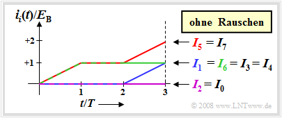
| − | $\text{ | + | $\text{Example 4:}$ The graph shows the continuous integral values, again assuming the actual transmitted signal $s_5(t)$ and the noise-free case. The corresponding bipolar equivalent was considered in [[Digital_Signal_Transmission/Optimal_Receiver_Strategies#Representation_of_the_correlation_receiver_in_the_tree_diagram|"Example 2"]]. |
| − | [[File:Dig_T_3_7_S5D_version2.png|right|frame| | + | [[File:Dig_T_3_7_S5D_version2.png|right|frame|Tree diagram of the correlation receiver (unipolar)|class=fit]] |
| − | + | For this example, the following comparison values result, each normalized to $E_{\rm B}$: | |
:$$I_5 = I_7 = 2, \hspace{0.2cm}I_1 = I_3 = I_4= I_6 = 1 \hspace{0.2cm}, | :$$I_5 = I_7 = 2, \hspace{0.2cm}I_1 = I_3 = I_4= I_6 = 1 \hspace{0.2cm}, | ||
\hspace{0.2cm}I_0 = I_2 = 0 | \hspace{0.2cm}I_0 = I_2 = 0 | ||
| Line 221: | Line 221: | ||
\hspace{0.05cm}.$$ | \hspace{0.05cm}.$$ | ||
| − | + | This means: | |
| − | * | + | *When compared in terms of maximum $I_i$ values, the source symbol sequences $Q_5$ and $Q_7$ would be equivalent. |
| − | * | + | *On the other hand, if the different energies $(E_5 = 2, \ E_7 = 3)$ are taken into account, the decision is clearly in favor of the sequence $Q_5$ because of $W_5 > W_7$. |
| − | * | + | *The correlation receiver according to $W_i = I_i- E_i/2$ therefore decides correctly on $s(t) = s_5(t)$ even with unipolar signaling. }}<br> |
| − | == | + | == Exercises for the chapter== |
<br> | <br> | ||
| − | [[Aufgaben: | + | [[Aufgaben:Exercise_3.09:_Correlation_Receiver_for_Unipolar_Signaling|Exercise 3.09: Correlation Receiver for Unipolar Signaling]] |
| − | [[Aufgaben: | + | [[Aufgaben:Exercise_3.10:_Maximum_Likelihood_Tree_Diagram|Exercise 3.10: Maximum Likelihood Tree Diagram]] |
{{Display}} | {{Display}} | ||
Revision as of 11:17, 31 May 2022
Contents
- 1 Considered scenario and prerequisites
- 2 MAP and Maximum–Likelihood decision rule
- 3 Maximum likelihood decision for Gaussian noise
- 4 Matched filter receiver vs. correlation receiver
- 5 Representation of the correlation receiver in the tree diagram
- 6 Correlation receiver with unipolar signaling
- 7 Exercises for the chapter
Considered scenario and prerequisites
All digital receivers described so far always make symbolwise decisions. If, on the other hand, several symbols are decided simultaneously, statistical bindings between the received signal samples can be taken into account during detection, which results in a lower error probability – but at the cost of an additional runtime.
In this – partly also in the next chapter – the following transmission model is assumed:
Compared to the last two chapters, the following differences arise:
- $Q \in \{Q_i\}$ with $i = 0$, ... , $M-1$ denotes a time-constrained source symbol sequence $\langle q_\nu \rangle$ whose symbols are to be jointly decided by the optimal receiver.
- If $Q$ describes a sequence of $N$ redundancy-free binary symbols, set $M = 2^N$. On the other hand, if the decision is symbolwise, $M$ specifies the level number of the digital source.
- In the above model, any channel distortions are added to the transmitter and are thus already included in the basic pulse $g_s(t)$ and the signal $s(t)$. This measure is only for a simpler representation and is not a restriction.
- Knowing the currently applied received signal $s(t)$, the optimal receiver searches from the set $\{Q_0$, ... , $Q_{M-1}\}$ of the possible source symbol sequences, the receiver searches for the most likely transmitted sequence $Q_j$ and outputs this as a sink symbol sequence $V$.
- Before the actual decision algorithm, a numerical value $W_i$ must be derived from the received signal $r(t)$ for each possible sequence $Q_i$ by suitable signal preprocessing. The larger $W_i$ is, the greater the inference probability that $Q_i$ was transmitted.
- Signal preprocessing must provide for the necessary noise power limitation and – in the case of strong channel distortions – for sufficient pre-equalization of the resulting intersymbol interferences. In addition, preprocessing also includes sampling for time discretization.
MAP and Maximum–Likelihood decision rule
The (unconstrained) optimal receiver is called the MAP receiver, where "MAP" stands for "Maximum–a–posteriori".
$\text{Definition:}$ The MAP receiver determines the $M$ inference probabilities ${\rm Pr}\big[Q_i \hspace{0.05cm}\vert \hspace{0.05cm}r(t)\big]$ and sets the output sequence $V$ according to the decision rule, where the index is: $i = 0$, ... , $M-1$ as well as $i \ne j$:
- $${\rm Pr}\big[Q_j \hspace{0.05cm}\vert \hspace{0.05cm} r(t)\big] > {\rm Pr}\big[Q_i \hspace{0.05cm}\vert \hspace{0.05cm} r(t)\big] \hspace{0.05cm}.$$
The "inference probability" ${\rm Pr}\big[Q_i \hspace{0.05cm}\vert \hspace{0.05cm} r(t)\big]$ indicates the probability with which the sequence $Q_i$ was sent when the received signal $r(t)$ is present at the decision. Using "Bayes' theorem", this probability can be calculated as follows:
- $${\rm Pr}\big[Q_i \hspace{0.05cm}|\hspace{0.05cm} r(t)\big] = \frac{ {\rm Pr}\big[ r(t)\hspace{0.05cm}|\hspace{0.05cm} Q_i \big] \cdot {\rm Pr}\big[Q_i]}{{\rm Pr}[r(t)\big]} \hspace{0.05cm}.$$
The MAP decision rule can thus be reformulated or simplified as follows: Let the sink symbol sequence $V = Q_j$ if for all $i \ne j$ holds:
- $$\frac{ {\rm Pr}\big[ r(t)\hspace{0.05cm}|\hspace{0.05cm} Q_j \big] \cdot {\rm Pr}\big[Q_j)}{{\rm Pr}\big[r(t)\big]} > \frac{ {\rm Pr}\big[ r(t)\hspace{0.05cm}|\hspace{0.05cm} Q_i\big] \cdot {\rm Pr}\big[Q_i\big]}{{\rm Pr}\big[r(t)\big]}\hspace{0.3cm} \Rightarrow \hspace{0.3cm} {\rm Pr}\big[ r(t)\hspace{0.05cm}|\hspace{0.05cm} Q_j\big] \cdot {\rm Pr}\big[Q_j\big]> {\rm Pr}\big[ r(t)\hspace{0.05cm}|\hspace{0.05cm} Q_i \big] \cdot {\rm Pr}\big[Q_i\big] \hspace{0.05cm}.$$
A further simplification of this MAP decision rule leads to the ML receiver, where "ML" stands for "maximum likelihood".
$\text{Definition:}$ The maximum likelihood receiver – abbreviated ML – decides according to the conditional forward probabilities ${\rm Pr}\big[r(t)\hspace{0.05cm} \vert \hspace{0.05cm}Q_i \big]$ and sets the output sequence $V = Q_j$ if for all $i \ne j$ holds:
- $${\rm Pr}\big[ r(t)\hspace{0.05cm} \vert\hspace{0.05cm} Q_j \big] > {\rm Pr}\big[ r(t)\hspace{0.05cm} \vert \hspace{0.05cm} Q_i\big] \hspace{0.05cm}.$$
A comparison of these two definitions shows:
- For equally probable source symbols, the ML receiver and the MAP receiver use the same decision rules; thus, they are equivalent.
- For symbols that are not equally probable, the ML receiver is inferior to the MAP receiver because it does not use all the available information for detection.
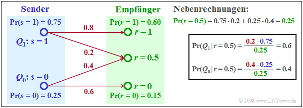
$\text{Example 1:}$ To illustrate ML and MAP decision rule, we now construct a very simple example with only two source symbols $(M = 2)$.
- The two possible symbols $Q_0$ and $Q_1$ are represented by the transmitted signals $s = 0$ and $s = 1$.
- The received signal can – for whatever reason – take three different values, namely $r = 0$, $r = 1$ and additionally $r = 0.5$.
The received values $r = 0$ and $r = 1$ will be assigned to the transmitter values $s = 0 \ (Q_0)$ and $s = 1 \ (Q_1)$, respectively, by both the ML and MAP decisions. In contrast, the decisions will give a different result with respect to the received value $r = 0.5$:
- The maximum likelihood decision rule leads to the source symbol $Q_0$, because of
- $${\rm Pr}\big [ r= 0.5\hspace{0.05cm}\vert\hspace{0.05cm} Q_0\big ] = 0.4 > {\rm Pr}\big [ r= 0.5\hspace{0.05cm} \vert \hspace{0.05cm} Q_1\big ] = 0.2 \hspace{0.05cm}.$$
- The MAP decision, on the other hand, leads to the source symbol $Q_1$, since according to the secondary calculation in the graph:
- $${\rm Pr}\big [Q_1 \hspace{0.05cm}\vert\hspace{0.05cm} r= 0.5\big ] = 0.6 > {\rm Pr}\big [Q_0 \hspace{0.05cm}\vert\hspace{0.05cm} r= 0.5\big ] = 0.4 \hspace{0.05cm}.$$
Maximum likelihood decision for Gaussian noise
We now assume that the received signal $r(t)$ is additively composed of a useful signal $s(t)$ and a noise component $n(t)$, where the noise is assumed to be Gaussian distributed and white ⇒ "AWGN noise":
- $$r(t) = s(t) + n(t) \hspace{0.05cm}.$$
Any channel distortions are already applied to the signal $s(t)$ for simplicity.
The necessary noise power limitation is realized by an integrator; this corresponds to an averaging of the noise values in the time domain. If one limits the integration interval to the range $t_1$ to $t_2$, one can derive a quantity $W_i$ for each source symbol sequence $Q_i$, which is a measure for the conditional probability ${\rm Pr}\big [ r(t)\hspace{0.05cm} \vert \hspace{0.05cm} Q_i\big ] $:
- $$W_i = \int_{t_1}^{t_2} r(t) \cdot s_i(t) \,{\rm d} t - {1}/{2} \cdot \int_{t_1}^{t_2} s_i^2(t) \,{\rm d} t= I_i - {E_i}/{2} \hspace{0.05cm}.$$
This decision variable $W_i$ can be derived using the $k$–dimensionial "joint probability density" of the noise $($with $k \to \infty)$ and some boundary crossings. The result can be interpreted as follows:
- Integration is used for noise power reduction by averaging. If $N$ binary symbols are decided simultaneously by the maximum likelihood detector, set $t_1 = 0 $ and $t_2 = N \cdot T$ for distortion-free channel.
- The first term of the above decision variable $W_i$ is equal to the "energy cross-correlation function" formed over the finite time interval $NT$ between $r(t)$ and $s_i(t)$ at the point $\tau = 0$:
- $$I_i = \varphi_{r, \hspace{0.08cm}s_i} (\tau = 0) = \int_{0}^{N \cdot T}r(t) \cdot s_i(t) \,{\rm d} t \hspace{0.05cm}.$$
- The second term gives the half energy of the considered useful signal $s_i(t)$ to be subtracted. The energy is equal to the ACF of the useful signal at the point $\tau = 0$:
- \[E_i = \varphi_{s_i} (\tau = 0) = \int_{0}^{N \cdot T} s_i^2(t) \,{\rm d} t \hspace{0.05cm}.\]
- In case of distorting channel the impulse response $h_{\rm K}(t)$ is not Dirac-shaped, but for example extended to the range $-T_{\rm K} \le t \le +T_{\rm K}$. In this case, $t_1 = -T_{\rm K}$ and $t_2 = N \cdot T +T_{\rm K}$ must be used for the two integration limits.
Matched filter receiver vs. correlation receiver
There are various circuit implementations of the maximum likelihood receiver.
For example, the required integrals can be obtained by linear filtering and subsequent sampling. This realization form is called matched filter receiver, because here the impulse responses of the $M$ parallel filters have the same shape as the useful signals $s_0(t)$, ... , $s_{M-1}(t)$.
- The $M$ decision variables $I_i$ are then equal to the convolution products $r(t) \star s_i(t)$ at time $t= 0$.
- For example, the "optimal binary receiver" described in detail in the chapter "Optimization of Baseband Transmission Systems" allows a maximum likelihood decision with ML parameters $M = 2$ and $N = 1$.
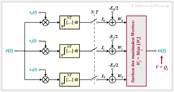
A second form of realization is provided by the correlation receiver according to the following graph.
One recognizes from this block diagram for the indicated parameters:
- The drawn correlation receiver forms a total of $M = 8$ cross-correlation functions between the received signal $r(t) = s_k(t) + n(t)$ and the possible transmitted signals $s_i(t), \ i = 0$, ... , $M-1$. The following description assumes that the useful signal $s_k(t)$ has been transmitted.
- The correlation receiver now searches for the maximum value $W_j$ of all correlation values and outputs the corresponding sequence $Q_j$ as a sink symbol sequence $V$. Formally, the ML decision rule can be expressed as follows:
- $$V = Q_j, \hspace{0.2cm}{\rm falls}\hspace{0.2cm} W_i < W_j \hspace{0.2cm}{\rm for}\hspace{0.2cm} {\rm all}\hspace{0.2cm} i \ne j \hspace{0.05cm}.$$
- If we further assume that all transmitted signals $s_i(t)$ have exactly the same energy, we can dispense with the subtraction of $E_i/2$ in all branches. In this case, the following correlation values are compared $(i = 0$, ... , $M-1)$:
- \[I_i = \int_{0}^{NT} s_j(t) \cdot s_i(t) \,{\rm d} t + \int_{0}^{NT} n(t) \cdot s_i(t) \,{\rm d} t \hspace{0.05cm}.\]
- With high probability, $I_j = I_k$ is larger than all other comparison values $I_{j \ne k}$. However, if the noise $n(t)$ is too large, the correlation receiver will also make a wrong decision.
Representation of the correlation receiver in the tree diagram
Let us illustrate the operation of the correlation receiver in the tree diagram, where the $2^3 = 8$ possible source symbol sequences $Q_i$ of length $N = 3$ are represented by bipolar rectangular transmitted signals $s_i(t)$:
The possible symbol sequences $Q_0 = \rm LLL$, ... , $Q_7 = \rm HHH$ and the associated transmitted signals $s_0(t)$, ... , $s_7(t)$ are listed above.
- Due to the bipolar amplitude coefficients and the rectangular shape all signal energies are equal: $E_0 = \text{...} = E_7 = N \cdot E_{\rm B}$, where $E_{\rm B}$ indicates the energy of a single pulse of duration $T$.
- Therefore, subtraction of the $E_i/2$ term in all branches can be omitted ⇒ a decision based on the correlation values $I_i$ gives equally reliable results as maximizing the corrected values $W_i$.
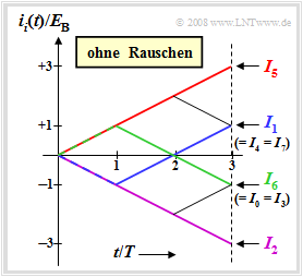
$\text{Example 2:}$ The graph shows the continuous integral values, assuming the actually transmitted signal $s_5(t)$ and the noise-free case. For this case, the time-dependent integral values and the integral end values are valid:
- $$i_i(t) = \int_{0}^{t} r(\tau) \cdot s_i(\tau) \,{\rm d} \tau = \int_{0}^{t} s_5(\tau) \cdot s_i(\tau) \,{\rm d} \tau \hspace{0.3cm} \Rightarrow \hspace{0.3cm}I_i = i_i(3T). $$
The graph can be interpreted as follows:
- Because of the rectangular shape of the signals $s_i(t)$, all function curves $i_i(t)$ are rectilinear. The end values normalized to $E_{\rm B}$ are $+3$, $+1$, $-1$ and $-3$.
- The maximum final value is $I_5 = 3 \cdot E_{\rm B}$ (red waveform), since signal $s_5(t)$ was actually sent. Without noise, the correlation receiver thus naturally always makes the correct decision.
- The blue curve $i_1(t)$ leads to the final value $I_1 = -E_{\rm B} + E_{\rm B}+ E_{\rm B} = E_{\rm B}$, since $s_1(t)$ differs from $s_5(t)$ only in the first bit. The comparison values $I_4$ and $I_7$ are also equal to $E_{\rm B}$.
- Since $s_0(t)$, $s_3(t)$ and $s_6(t)$ differ from the transmitted $s_5(t)$ in two bits, $I_0 = I_3 = I_6 =-E_{\rm B}$. The green curve shows $s_6(t)$ initially increasing (first bit matches) and then decreasing over two bits.
- The purple curve leads to the final value $I_2 = -3 \cdot E_{\rm B}$. The corresponding signal $s_2(t)$ differs from $s_5(t)$ in all three symbols and $s_2(t) = -s_5(t)$ holds.
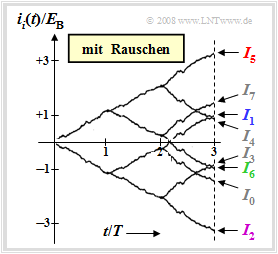
$\text{Example 3:}$ The graph for this example describes the same situation as $\text{Example 2}$, but now the received signal $r(t) = s_5(t)+ n(t)$ is assumed. The variance of the AWGN noise $n(t)$ here is $\sigma_n^2 = 4 \cdot E_{\rm B}/T$.
One can see from this graph compared to the noise-free case:
- The function curves are now no longer straight due to the noise component $n(t)$ and there are also slightly different final values than without noise.
- In the considered example, however, the correlation receiver decides correctly with high probability, since the difference between $I_5$ and the second larger value $I_7$ is relatively large with $1.65\cdot E_{\rm B}$.
- However, the error probability in the example considered here is not better than that of the matched filter receiver with symbolwise decision.
- In accordance with the chapter "Optimization of Baseband Transmission Systems", the following also applies here:
- $$p_{\rm S} = {\rm Q} \left( \sqrt{ {2 \cdot E_{\rm B} }/{N_0} }\right) = {1}/{2} \cdot {\rm erfc} \left( \sqrt{ { E_{\rm B} }/{N_0} }\right) \hspace{0.05cm}.$$
$\text{Conclusion:}$
- If the input signal does not have statistical bindings as in $\text{Example 2}$, there is no improvement by joint decision of $N$ symbols over symbolwise decision.
- In the presence of statistical bindings, the joint decision of $N$ symbols noticeably reduces the error probability compared to $p_{\rm S} = {\rm Q} \left( \sqrt{ {2 \cdot E_{\rm B} }/{N_0} }\right)$ (valid for symbolwise decision), since the maximum likelihood receiver takes the bindings into account.
- Such bindings can be either deliberately created by transmission-side coding (see $\rm LNTwww$ book "Channel Coding") or unintentionally caused by (linear) channel distortions.
- In the presence of such intersymbol interference, the calculation of the error probability is much more difficult. However, comparable approximations as for the Viterbi receiver can be given, which are given at the "end of the next chapter".
Correlation receiver with unipolar signaling
So far, we have always assumed binary bipolar signaling when describing the correlation receiver:
- $$a_\nu = \left\{ \begin{array}{c} +1 \\ -1 \\ \end{array} \right.\quad \begin{array}{*{1}c} {\rm{f\ddot{u}r}} \\ {\rm{for}} \\ \end{array}\begin{array}{*{20}c} q_\nu = \mathbf{H} \hspace{0.05cm}, \\ q_\nu = \mathbf{L} \hspace{0.05cm}. \\ \end{array}$$
Now we consider the case of binary unipolar digital signaling holds:
- $$a_\nu = \left\{ \begin{array}{c} 1 \\ 0 \\ \end{array} \right.\quad \begin{array}{*{1}c} {\rm{for}} \\ {\rm{for}} \\ \end{array}\begin{array}{*{20}c} q_\nu = \mathbf{H} \hspace{0.05cm}, \\ q_\nu = \mathbf{L} \hspace{0.05cm}. \\ \end{array}$$
The $2^3 = 8$ possible source symbol sequences $Q_i$ of length $N = 3$ are now represented by unipolar rectangular transmitted signals $s_i(t)$. Listed below are the symbol sequences $Q_0 = \rm LLL$, ... , $Q_7 = \rm HHH$ and the transmitted signals $s_0(t)$, ... , $s_7(t)$.
By comparing with the "corresponding table" for bipolar signaling, one can see:
- Due to the unipolar amplitude coefficients, the signal energies $E_i$ are now different, for example $E_0 = 0$ and $E_7 = 3 \cdot E_{\rm B}$.
- Here the decision based on the integral end values $I_i$ does not lead to the correct result.
- Instead, the corrected comparison values $W_i = I_i- E_i/2$ must now be used.
$\text{Example 4:}$ The graph shows the continuous integral values, again assuming the actual transmitted signal $s_5(t)$ and the noise-free case. The corresponding bipolar equivalent was considered in "Example 2".
For this example, the following comparison values result, each normalized to $E_{\rm B}$:
- $$I_5 = I_7 = 2, \hspace{0.2cm}I_1 = I_3 = I_4= I_6 = 1 \hspace{0.2cm}, \hspace{0.2cm}I_0 = I_2 = 0 \hspace{0.05cm},$$
- $$W_5 = 1, \hspace{0.2cm}W_1 = W_4 = W_7 = 0.5, \hspace{0.2cm} W_0 = W_3 =W_6 =0, \hspace{0.2cm}W_2 = -0.5 \hspace{0.05cm}.$$
This means:
- When compared in terms of maximum $I_i$ values, the source symbol sequences $Q_5$ and $Q_7$ would be equivalent.
- On the other hand, if the different energies $(E_5 = 2, \ E_7 = 3)$ are taken into account, the decision is clearly in favor of the sequence $Q_5$ because of $W_5 > W_7$.
- The correlation receiver according to $W_i = I_i- E_i/2$ therefore decides correctly on $s(t) = s_5(t)$ even with unipolar signaling.
Exercises for the chapter
Exercise 3.09: Correlation Receiver for Unipolar Signaling
Exercise 3.10: Maximum Likelihood Tree Diagram

