Channel Coding/Bounds for Block Error Probability

1. Channel Coding
2. Binary Block Codes for Channel Coding
3. Bounds for Block Error Probability

• Previous page
• Next page

• Previous page
• Next page

Distance spectrum of a linear code

We further assume a linear and binary  $(n, \hspace{0.05cm} k)$ block code  $\mathcal{C}$.  A major goal of code design is to keep the  "block error probability"  ${\rm Pr}(\underline{u} \ne \underline{v}) = {\rm Pr}(\underline{z} \ne \underline{x})$  as low as possible.  This is achieved by,  among other things

• the minimum distance  $d_{\rm min}$  between two code words  $\underline{x}$  and  $\underline{x}\hspace{0.05cm}'$  is as large as possible,  so that one can correct up to  $t = ⌊(d_{\rm min}-1)/2⌋$  bit errors;
  

• at the same time this minimum distance  $d_{\rm min}$  occurs as rarely as possible,  given all the allowed code words.
  
  

$\text{Definition:}$  We denote the  number  of code words  $\underline{x}\hspace{0.05cm}' \in \mathcal{C}$  with Hamming distance  $i$  from the considered code word  $\underline{x}$  of the same code  $\mathcal{C}$  with  $W_i(\underline{x})$,  where holds:

\[W_i(\underline{x}) = \big \vert \hspace{0.05cm} \left \{ \underline{x} \hspace{0.05cm}, \underline{x}{\hspace{0.05cm}' \in \hspace{0.05cm} \mathcal{C} } \hspace{0.1cm}\vert\hspace{0.1cm} d_{\rm H}(\underline{x} \hspace{0.05cm}, \hspace{0.1cm}\underline{x}\hspace{0.05cm}' ) = i \right \} \hspace{0.05cm} \big \vert\hspace{0.05cm}.\]

• The amount strokes of the absolute value here denote the number of code words  $\underline{x}\hspace{0.05cm}'$, that satisfy the condition  $d_{\rm H}(\underline{x} \hspace{0.05cm}, \hspace{0.1cm}\underline{x}\hspace{0.05cm}' ) = i $. 

• This value is also called  "multiplicity".

$\text{Example 1:}$  We consider the  $(5, \, 2)$ block code  $\mathcal{C}$  with generator matrix

Hamming distances between all code words

\[{ \boldsymbol{\rm G} } = \begin{pmatrix} 1 &0 &1 &1 &0 \\ 0 &1 &0 &1 &1 \end{pmatrix} \hspace{0.05cm}.\]

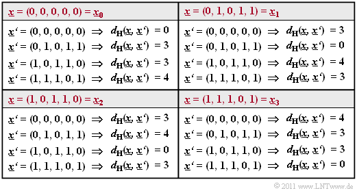
The table shows the Hamming distances

• between all code words  $\underline{x}_i$

• to the reference words  $\underline{x}_0$, ... , $\underline{x}_3$.

One recognizes:   Independently of the reference word  $\underline{x}_i$  holds:

\[W_0 = 1 \hspace{0.05cm}, \hspace{0.5cm}W_1 = W_2 = 0 \hspace{0.05cm},\hspace{0.5cm} W_3 = 2 \hspace{0.05cm},\hspace{0.5cm} W_4 = 1\]

\[ \Rightarrow\hspace{0.3cm} d_{\rm min} = 3\hspace{0.05cm}.\]

Not only in this example,  but in any linear code,  the same multiplicities  $W_i$  result for each code word.  Furthermore,  since the all-zero word   $\underline{0} = (0, 0,\text{ ...} \hspace{0.05cm}, 0)$   is part of every linear binary code,  the above definition can also be formulated as follows:

$\text{Definition:}$  The  distance spectrum  of a linear binary  $(n, \hspace{0.03cm} k)$  block code is the set   $\{W_i \}$  with  $i = 0,\ 1,$ ... ,  $n$. 

• Here,  $W_i$  gives the number of code words  $\underline{x} \in \mathcal{C}$  with Hamming weight  $w_{\rm H}(\underline{x}) = i$.

• Often one describes the set  $\hspace{0.05cm}\{W_i \}\hspace{0.05cm}$  also as a polynomial with a pseudo-variable  $X$:

\[\left \{ \hspace{0.05cm} W_i \hspace{0.05cm} \right \} \hspace{0.3cm} \Leftrightarrow \hspace{0.3cm} W(X) = \sum_{i=0 }^{n} W_i \cdot X^{i} = W_0 + W_1 \cdot X + W_2 \cdot X^{2} + ... \hspace{0.05cm} + W_n \cdot X^{n}\hspace{0.05cm}.\]

• $W(X)$  is also called the   weight enumerator function.

• For example,  the weight enumerator function of the  $(5, \hspace{0.02cm} 2)$  code  $\mathcal{C} = \left \{ \hspace{0.05cm}(0, 0, 0, 0, 0) \hspace{0.05cm},\hspace{0.15cm} (0, 1, 0, 1, 1) \hspace{0.05cm},\hspace{0.15cm}(1, 0, 1, 1, 0) \hspace{0.05cm},\hspace{0.15cm}(1, 1, 1, 0, 1) \hspace{0.05cm} \right \}$  of  $\text{Example 1}$:

\[W(X) = 1 + 2 \cdot X^{3} + X^{4}\hspace{0.05cm}.\]

• As can be seen for the  $(7, \hspace{0.02cm}4, \hspace{0.02cm}3)$ Hamming code from the  "table of its code words":

\[W(X) = 1 + 7 \cdot X^{3} + 7 \cdot X^{4} + X^{7}\hspace{0.05cm}.\]

• The transformation of the distance spectrum  $\hspace{0.01cm}\{W_i \}\hspace{0.01cm}$  into the weight enumerator function  $W(X)$  also offers great numerical advantages in some exercises.  For example,  if the weight enumerator function  $W(X)$  of a  $(n, \hspace{0.03cm} k)$–Block Codes  $\mathcal{C}$  is known,  then for the corresponding  "dual"  $(n, \hspace{0.03cm} n-k)$  code  $\mathcal{C}_{\rm dual}$:

\[W_{\rm dual}(X) = \frac{(1+X)^n}{2^k} \cdot W \left ( \frac{1-X}{1+X} \right )\hspace{0.05cm}.\]

$\text{Example 2:}$  The weight enumerator function  $W(X)$  of the  "single parity–check codes"  with   $n = 6$,  $k = 5$   ⇒   $\text{SPC (6, 5)}$  is obtained by comparing all  $2^5 = 32$  code words with the all-zero word:

\[W_{\rm SPC\hspace{0.03cm}(6,\hspace{0.08cm}5)}(X) = 1 + 15 \cdot X^{2} + 15 \cdot X^{4} + X^{6}\hspace{0.05cm}.\]

Considering the above equation, you get the same result much faster:

• The dual code to  $\text{SPC (6, 5)}$  is the  "repetition code"  $\text{RC (6, 1)}$  with only two code words  $(0, 0, 0, 0, 0, 0)$  and  $(1, 1, 1, 1, 1, 1)$:

\[W_{\rm RC\hspace{0.03cm}(6,\hspace{0.08cm}1)}(X) = 1 + X^{6}\hspace{0.05cm}.\]

• From this it follows for the weight enumerator function of the  $\text{SPC (6, 5)}$  according to the above equation with  $k = 1$:

\[W_{\rm SPC\hspace{0.03cm}(6,\hspace{0.08cm}5)}(X) = \frac{(1+X)^6}{2^1} \cdot W \left [1 \hspace{-0.05cm}+\hspace{-0.05cm} \left ( \frac {1\hspace{-0.05cm}-\hspace{-0.05cm}X}{1\hspace{-0.05cm}+\hspace{-0.05cm}X}\right )^6 \right ] = 1/2 \cdot \big [( 1\hspace{-0.05cm}+\hspace{-0.05cm}X) ^6 \hspace{-0.05cm}+\hspace{-0.05cm} ( 1-X) ^6 \big ] = 1 \hspace{-0.05cm}+\hspace{-0.05cm} 15 \cdot X^{2} \hspace{-0.05cm}+\hspace{-0.05cm} 15 \cdot X^{4} \hspace{-0.05cm}+\hspace{-0.05cm} X^{6}\hspace{0.05cm}.\]

Union Bound of the block error probability

We consider as in  $\text{Example 1}$  the distance spectrum of the  $(5, \hspace{0.02cm} 2)$  block code  $\mathcal{C} = \{\underline{x}_0, \underline{x}_1, \underline{x}_2, \underline{x}_3 \}$   and assume that the code word  $\underline{x}_0$  has been sent.  The graphic illustrates the situation.

• In the error-free case,  the code word estimator would then return  $\underline{z} = \underline{x}_0$. 

• Otherwise,  a block error would occur  (that is,   $\underline{z} \ne \underline{x}_0$  and accordingly  $\underline{v} \ne \underline{u}_0)$  with probability

Derivation of the Union Bound

$${\rm Pr(block\:error)} = {\rm Pr}\left (\big [\underline{x}_{\hspace{0.02cm}0} \hspace{-0.07cm}\mapsto \hspace{-0.07cm}\underline{x}_{\hspace{0.02cm}1}\big ] \hspace{-0.07cm}\cup\hspace{-0.07cm}\big [\underline{x}_{\hspace{0.02cm}0} \hspace{-0.07cm}\mapsto \hspace{-0.07cm} \underline{x}_{\hspace{0.02cm}2}\big ] \hspace{-0.07cm}\cup\hspace{-0.07cm}\big [\underline{x}_{\hspace{0.02cm}0} \hspace{-0.07cm}\mapsto \hspace{-0.07cm} \underline{x}_{\hspace{0.02cm}3}\big ] \right ).$$

⇒  The event  "falsification from   $\underline{x}_0$   to  $\underline{x}_1$"  occurs for a given received word   $\underline{y}$   according to the  "maximum likelihood block-wise decision rule"  exactly when for the conditional probability density function holds:

\[\big [\underline{x}_{\hspace{0.02cm}0} \mapsto \underline{x}_{\hspace{0.02cm}1}\big ] \hspace{0.3cm} \Leftrightarrow \hspace{0.3cm} f(\underline{x}_{\hspace{0.02cm}0}\hspace{0.02cm} | \hspace{0.05cm}\underline{y}) < f(\underline{x}_{\hspace{0.02cm}1}\hspace{0.02cm} | \hspace{0.05cm}\underline{y}) \hspace{0.05cm}.\]

⇒   Since the events  $\big [\underline{x}_{\hspace{0.02cm}0} \mapsto \underline{x}_{\hspace{0.02cm}1}\big ] $,  $\big [\underline{x}_{\hspace{0.02cm}0} \mapsto \underline{x}_{\hspace{0.02cm}2}\big ] $,  $\big [\underline{x}_{\hspace{0.02cm}0} \mapsto \underline{x}_{\hspace{0.02cm}3}\big ] $  are not necessarily  "disjoint"   (which would thus be mutually exclusive),  the  "probability of the union set"  is less than or equal to the sum of the individual probabilities:

\[{\rm Pr(block\:error)} \le {\rm Pr}\big [\underline{x}_{\hspace{0.02cm}0} \mapsto \underline{x}_{\hspace{0.02cm}1}\big ] \hspace{0.05cm}+\hspace{0.05cm}{\rm Pr}\big [\underline{x}_{\hspace{0.02cm}0} \mapsto \underline{x}_{\hspace{0.02cm}2}\big ] \hspace{0.05cm}+ \hspace{0.05cm}{\rm Pr}\big [\underline{x}_{\hspace{0.02cm}0} \mapsto \underline{x}_{\hspace{0.02cm}3}\big ] \hspace{0.05cm}.\]

1. One calls this upper bound for the block error probability the  Union Bound.
2. This was already used in the chapter  "Approximation of the error probability"  of the book  "Digital Signal Transmission".
   

We generalize now and formalize these results under the assumption that both  $\underline{x}$  and  $\underline{x}\hspace{0.05cm}'$  belong to the code  $\mathcal{C}$ .

$\text{Then the following calculation rules apply:}$ 

• $\rm Block\:error\:probability$:

$${\rm Pr(block\:error)} = {\rm Pr} \left ( \bigcup_{\underline{x}\hspace{0.05cm}' \ne \underline{x} } \hspace{0.15cm}\big [\underline{x} \mapsto \underline{x}\hspace{0.05cm}'\big] \right )\hspace{0.05cm},$$

• Upper bound   ⇒   $\text{Union Bound}$:

$${\rm Pr(Union \hspace{0.15cm}Bound)} \le \sum_{\underline{x}\hspace{0.05cm}' \ne \underline{x} } \hspace{0.15cm} {\rm Pr}\big[\underline{x} \mapsto \underline{x}\hspace{0.05cm}'\big] \hspace{0.05cm},$$

• $\text{Pairwise error probability}$  (according to the maximum-a- posteriori resp. maximum likelihood criterion):

$${\rm Pr}\hspace{0.02cm}\big[\underline{x} \mapsto \underline{x}\hspace{0.05cm}'\big] = {\rm Pr} \big [ p(\underline{x}\hspace{0.05cm}\vert \hspace{0.05cm}\underline{y}) \le p(\underline{x}\hspace{0.05cm}'\hspace{0.05cm} \vert \hspace{0.05cm}\underline{y}) \big ] \hspace{0.05cm}.$$

On the next pages,  these results are applied to different channels.

Union Bound for the BSC model

We further consider the exemplary  $(5, \hspace{0.02cm} 2)$ code: 

BSC model and maximum likelihood detection

$$\mathcal{C} = \left \{ \hspace{0.05cm}(0, 0, 0, 0, 0) \hspace{0.05cm},\hspace{0.15cm} (0, 1, 0, 1, 1) \hspace{0.05cm},\hspace{0.15cm}(1, 0, 1, 1, 0) \hspace{0.05cm},\hspace{0.15cm}(1, 1, 1, 0, 1) \hspace{0.05cm} \right \}.$$

For the digital channel we use the  "BSC model"  ("Binary Symmetric Channel"):

\[{\rm Pr}(y = 1 \hspace{0.05cm} | \hspace{0.05cm}x = 0 ) = {\rm Pr}(y = 0 \hspace{0.05cm} | \hspace{0.05cm}x = 1 ) = {\rm Pr}(e = 1) = \varepsilon \hspace{0.05cm},\]

\[{\rm Pr}(y = 0 \hspace{0.05cm} | \hspace{0.05cm}x = 0 ) = {\rm Pr}(y = 1 \hspace{0.05cm} | \hspace{0.05cm}x = 1 ) = {\rm Pr}(e = 0) = 1 -\varepsilon \hspace{0.05cm}.\]

Then holds:

1. The code words  $\underline{x}_0 = (0, 0, 0, 0, 0)$  and  $\underline{x}_1 = (0, 1, 0, 1, 1)$  differ in  $d = 3$  bits;  $d$  indicates the "Hamming distance"  between  $\underline{x}_0$  and  $\underline{x}_1$.
2. An incorrect decoding result   $\big[\underline{x}_{\hspace{0.02cm}0} \mapsto \underline{x}_{\hspace{0.02cm}1}\big] $  is obtained whenever at least two of the three bits at bit positions 2, 4, and 5 are corrupted.
3. In contrast,maximum likelihood the bit positions 1 and 3 do not matter here,maximum likelihood since they are the same for  $\underline{x}_0$  and  $\underline{x}_1$.

Since the considered code can correct  $t = ⌊(d-1)/2⌋ = 1$  errors:

\[{\rm Pr}\big [\underline{x}_{\hspace{0.02cm}0} \mapsto \underline{x}_{\hspace{0.02cm}1}\big ] \hspace{-0.1cm} = \hspace{-0.1cm} \sum_{i=t+1 }^{d} {d \choose i} \cdot \varepsilon^{i} \cdot (1 - \varepsilon)^{d-i} = {3 \choose 2} \cdot \varepsilon^{2} \cdot (1 - \varepsilon) + {3 \choose 3} \cdot \varepsilon^{3} =3 \cdot \varepsilon^2 \cdot (1 - \varepsilon) + \varepsilon^3 = {\rm Pr}\big[\underline{x}_{\hspace{0.02cm}0} \mapsto \underline{x}_{\hspace{0.02cm}2}\big]\hspace{0.05cm}.\]

This takes into account that   $\underline{x}_0 = (0, 0, 0, 0, 0)$   and   $\underline{x}_2 = (1, 0, 1, 1, 0)$   also differ in three bit positions.

On the other hand,  the code words   $\underline{x}_0 = (0, 0, 0, 0, 0)$   and   $\underline{x}_3 = (1, 1, 1, 0, 1)$   differ in four bit positions:

• Wrong decoding of the block therefore certainly occurs if four or three bits are corrupted.

• A corruption of two bits results in a block error with  $50\%$  probability,  if one assumes a random decision for this  (last term).

\[{\rm Pr}\big[\underline{x}_{\hspace{0.02cm}0} \mapsto \underline{x}_{\hspace{0.02cm}3}\big] = \varepsilon^4 + 4 \cdot \varepsilon^3 \cdot (1 - \varepsilon) + {1}/{2} \cdot 6 \cdot \varepsilon^2 \cdot (1 - \varepsilon)^2 \hspace{0.05cm}.\]

• This results in the "Union Bound":

\[{\rm Pr(Union \hspace{0.15cm}Bound)} = {\rm Pr}\big[\underline{x}_{\hspace{0.02cm}0} \hspace{-0.02cm}\mapsto \hspace{-0.02cm}\underline{x}_{\hspace{0.02cm}1}\big] +{\rm Pr}\big[\underline{x}_{\hspace{0.02cm}0} \hspace{-0.02cm}\mapsto \hspace{-0.02cm} \underline{x}_{\hspace{0.02cm}2}] +{\rm Pr}[\underline{x}_{\hspace{0.02cm}0} \hspace{-0.02cm}\mapsto \hspace{-0.02cm} \underline{x}_{\hspace{0.02cm}3}\big] \ge {\rm Pr(block\hspace{0.15cm}error)} .\]

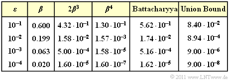
$\text{Example 3:}$  The table summarizes the results for different values of the BSC parameter  $\varepsilon$ .

Numeric Union Bound for the considered  $\text{(5, 2)}$ code

It is worth mentioning that the completely different probabilities to be calculated 

• ${\rm Pr}\big[\underline{x}_{\hspace{0.02cm}0} \hspace{-0.02cm}\mapsto \hspace{-0.02cm}\underline{x}_{\hspace{0.02cm}1}\big]=3 \cdot \varepsilon^2 \cdot (1 - \varepsilon) + \varepsilon^3 = {\rm Pr}\big[\underline{x}_{\hspace{0.02cm}0} \mapsto \underline{x}_{\hspace{0.02cm}2}\big]={\rm Pr}\big[\underline{x}_{\hspace{0.02cm}0} \hspace{-0.02cm}\mapsto \hspace{-0.02cm}\underline{x}_{\hspace{0.02cm}2}\big]\hspace{0.05cm},$ 

• ${\rm Pr}\big[\underline{x}_{\hspace{0.02cm}0} \hspace{-0.02cm}\mapsto \hspace{-0.02cm}\underline{x}_{\hspace{0.02cm}3}\big]= \varepsilon^4 + 4 \cdot \varepsilon^3 \cdot (1 - \varepsilon) + {1}/{2} \cdot 6 \cdot \varepsilon^2 \cdot (1 - \varepsilon)^2 \hspace{0.05cm},$ 

give exactly the same numerical result.

The upper bound according to Bhattacharyya

Another upper bound on the block error probability was given by  "Anil Kumar Bhattacharyya" :

\[{\rm Pr(block\:error)} \le W(X = \beta) -1 = {\rm Pr(Bhattacharyya)} \hspace{0.05cm}.\]

It should be noted that:

• $W(X)$  is the above defined  "weight enumerator function" characterizing the channel code used.
  

• The  "Bhattacharyya parameter"  $\beta$  identifies the digital channel.  For example:

\[\beta = \left\{ \begin{array}{c} \lambda \\ \sqrt{4 \cdot \varepsilon \cdot (1- \varepsilon)}\\ {\rm e}^{- R \hspace{0.05cm}\cdot \hspace{0.05cm}E_{\rm B}/N_0} \end{array} \right.\quad \begin{array}{*{1}c} {\rm for \hspace{0.15cm}BEC\hspace{0.15cm}model},\\ {\rm for \hspace{0.15cm}BSC\hspace{0.15cm}model}, \\ {\rm for\hspace{0.15cm}AWGN\hspace{0.15cm} model}. \end{array}\]

• The  "Bhattacharyya Bound"  is always  (and usually significantly)  above the curve for the "Union Bound". With the goal of finding a uniform bound for all channels,  much coarser estimates must be made here than for the  "Union Bound".
  
  

We restrict ourselves here to the  Bhattacharyya bound for the BSC model.

• For its pairwise error probability was derived in front:

\[{\rm Pr}\big[\underline{x}_{\hspace{0.02cm}0} \mapsto \underline{x}_{\hspace{0.02cm}1}\big] = \sum_{i= \left\lfloor (d-1)/2 \right\rfloor}^{d} {d \choose i} \cdot \varepsilon^{i} \cdot (1 - \varepsilon)^{d-i} = \sum_{i= \left\lceil d/2 \right\rceil }^{d} {d \choose i} \cdot \varepsilon^{i} \cdot (1 - \varepsilon)^{d-i}\hspace{0.05cm}.\]

Here,  $\varepsilon = {\rm Pr}(y = 1\hspace{0.04cm}|\hspace{0.04cm} x = 0) = {\rm Pr}(y = 0\hspace{0.04cm}|\hspace{0.04cm} x = 1)< 0.5$  denotes the BSC model,  and  $d = d_{\rm H}(\underline{x}_0,\, \underline{x}_1)$  indicates the Hamming distance between all code words.

• To arrive at the Bhattacharyya bound, the following estimates must be made:  For all  $i < d$  holds  $\varepsilon^{i} \cdot (1 - \varepsilon)^{d-i} \le (1 - \varepsilon)^{d/2}$:

\[{\rm Pr}\big[\underline{x}_{\hspace{0.02cm}0} \mapsto \underline{x}_{\hspace{0.02cm}1}\big] \le \big[\varepsilon \cdot (1 - \varepsilon)\big]^{d/2} \cdot \sum_{i= \left\lceil d/2 \right\rceil }^{d} {d \choose i} \hspace{0.05cm}.\]

• Change with respect to the lower limit of the indexing variable  $i$:

\[\sum_{i= \left\lceil d/2 \right\rceil }^{d} {d \choose i} \hspace{0.15cm} < \hspace{0.15cm} \sum_{i= 0 }^{d} {d \choose i} = 2^d\hspace{0.05cm}, \hspace{0.2cm}\beta = 2 \cdot \sqrt{\varepsilon \cdot (1 - \varepsilon)} \hspace{0.3cm} \Rightarrow \hspace{0.3cm} {\rm Pr}\big[\underline{x}_{\hspace{0.02cm}0} \mapsto \underline{x}_{\hspace{0.02cm}1}\big] = \beta^{d} \hspace{0.05cm}.\]

• Resort according to Hamming weights  $W_i$  $($Hamming distance  $d = i$  occurs  $W_i$  times$)$:

\[{\rm Pr(block\:error)} \hspace{0.1cm} \le \hspace{0.1cm} \sum_{i= 1 }^{n} W_i \cdot \beta^{i} = 1 + W_1 \cdot \beta + W_2 \cdot \beta^2 + \hspace{0.05cm}\text{ ...} \hspace{0.05cm}+ W_n \cdot \beta^n \hspace{0.05cm}.\]

• With the weight enumerator function  $W(X)= 1 + W_1 \cdot X + W_2 \cdot X^2 + \text{...} + W_n \cdot X^n$:

\[{\rm Pr(block\:error)} \le W(X = \beta) -1= {\rm Pr(Bhattacharyya)} \hspace{0.05cm}.\]

$\text{Example 4:}$  The table summarizes the Bhattacharyya results for different values of the BSC parameter  $\varepsilon$  valid for the  "example $\text{(5, 2)}$ code".

"Union Bound"  vs.  "Bhattacharyya Barrier"  valid for BSC model

• For this one applies:

$$W_0 = 1, \ \ W_1 = W_2 = 0, \ \ W_3 = 2, \ \ W_4 = 1$$

$$\Rightarrow\hspace{0.3cm} W(X) = 1 + 2 \cdot X^3 + X^4.$$

• Thus,  the Bhattacharyya bound can be calculated:

\[ {\rm Pr(Bhattacharyya)} = W(\beta) -1 = 2 \cdot \beta^3 + \beta^4\hspace{0.05cm}.\]

• This provides a  (often rough)  bound on the block error probability:

\[ {\rm Pr(block\:error)} \le {\rm Pr(Bhattacharyya)} \hspace{0.05cm}.\]

$\text{Conclusions:}$  Based on  "$\text{Example 3}$"  and  $\text{Example 4}$  (on this page)  for the simple  $\text{(5, 2)}$  block code,  though of little practical relevance,  and in anticipation of  $\text{example 5}$  (on the next page)  for the  $\text{(7, 4, 3)}$  Hamming code,  we summarize:

1. The block error probability of a coding system is often not analytically specifiable and must be determined by simulation.  The same applies to the bit error probability.
   
2. The  Union Bound  provides an upper bound for the block error probability.  For many applications  $($especially short codes$)$  the Union Bound is only slightly above the actual error probability.
   
3. The  Bhattacharyya Bound  for the BEC channel is about a factor  $2$  above the  Union Bound  – see  "Exercise 1.14".  For the BSC and the AWGN channel,  the gap is much larger.  The factor  $10$  (and more)  is not uncommon.
   
4. The Bhattacharyya Bound   ⇒   "$W(\beta) - 1$"   looks very simple at first sight.  Nevertheless,  one needs also here knowledge about the exact weight function  $W(\xi)$  of the code.
   
5. If the transmission channel  $($BEC,  BSC,  AWGN  or variations thereof$)$  and its parameters are known,  there is nothing to be said against using the  (more accurate)  "Union Bound"  as an upper bound for the block error probability.

Bounds for the (7, 4, 3) Hamming code at the AWGN channel

Finally,  we consider the block error probability and its bounds  $($"Union Bound"  and  "Bhattacharyya Bound")  for the following configuration:

1. AWGN channel,  characterized by the quotient  $E_{\rm B}/N_0$,
   
2. Hamming code  $\text{HC(7, 4, 3)}$   ⇒   rate  $R = 4/7$,   weight enumerator function  $W(X)-1 = 7 \cdot X^3 + 7 \cdot X^4 + X^7$,
   
3. "Soft Decision"  according to the maximum likelihood criterion.
   
   

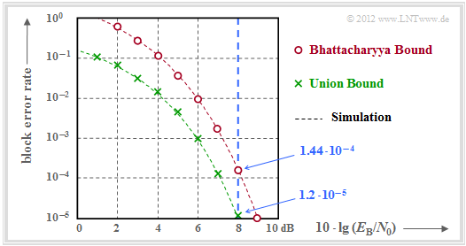
$\text{Example 5:}$  The results are summarized in the graph.

Block error probability and bounds of the  $\text{HC (7, 4, 3)}$

• In contrast to the graph in the section  "Coding gain – bit error rate with AWGN",  the  block error rate  is given here and not the bit error rate.

• Approximately,  the latter is smaller by the factor  $d_{\rm min}/k$  if,  as here  $d_{\rm min}< k$.  In the present example:  $d_{\rm min}/k = 0.75$.
  

• Only the points for integer  $\rm dB$  values were calculated.  The dashed lines were interpolated.

• The  (blue)  numerical values given on the right are for  (blue vertical)  $10 \cdot \lg \, E_{\rm B}/N_0 = 8 \, \rm dB$   ⇒   $E_{\rm B}/N_0 \approx 6.31$.

The green crosses mark the  "Union Bound".  For this applies:

\[{\rm Pr(block\:error)} \le \sum_{i= d_{\rm min} }^{n} W_i \cdot {\rm Q} \left ( \sqrt{i \cdot {2R \cdot E_{\rm B} }/{N_0} } \right ) \]

\[\Rightarrow \hspace{0.3cm}{\rm Pr(block\:error)} \approx 7 \cdot {\rm Q} (4.65) + 7 \cdot {\rm Q} (5.37) + {\rm Q} (7.10) = \]

\[\hspace{2.0cm} \approx 7 \cdot 1.66 \cdot 10^{-6} + 7 \cdot 3.93 \cdot 10^{-8}+ 10^{-9} = 1.2 \cdot 10^{-5} \hspace{0.05cm}.\]

• The numerical values make it clear that the Union Bound is essentially determined by the first term:

\[{\rm Pr(Union\hspace{0.15cm} Bound)} \approx W_{d_{\rm min} } \cdot {\rm Q} \left ( \sqrt{d_{\rm min} \cdot {2R \cdot E_{\rm B} }/{N_0} } \right ) = 1.16 \cdot 10^{-5} \hspace{0.05cm}.\]

• However,  this so-called  "Truncated Union Bound"  is no longer a true boundary for the block error probability in all applications,  but is to be understood as an approximation.
  

• The  "Bhattacharyya Bound"  is marked by red dots in the graph.  This is well above the Union Bound due to the highly simplified  "Chernoff–Rubin Bound" 

$${\rm Q}(x) \le {\rm e}^{-x^2/2}.$$

• For example,  for  $10 \cdot \lg \, E_{\rm B}/N_0 = 8 \, \rm dB$  with  $\beta = {\rm e}^{-R \hspace{0.05cm}\cdot \hspace{0.05cm}E_{\rm B}/N_0} \approx 0.027$  a more than tenfold value compared to the Union Bound:

\[{\rm Pr(Bhattacharyya)} = W(\beta) -1 = 7 \cdot \beta^3 + 7 \cdot \beta^4 + \beta^7 \approx 1.44 \cdot 10^{-4} \hspace{0.05cm}.\]

Exercises for the chapter

"Exercise 1.14: Bhattacharyya Bound for BEC"

"Exercise 1.15: Distance Spectra of HC (7, 4, 3) and HC (8, 4, 4)"

"Exercise 1.16: Block Error Probability Bounds for AWGN"

"Exercise 1.16Z: Bounds for the Gaussian Error Function"