Approximation of the Error Probability

1 Optimal decision with binary transmission
2 The special case of equally probable binary symbols
3 Error probability for symbols with equal probability
4 Optimal threshold for non-equally probable symbols
5 Decision regions in the non-binary case
6 Error probability calculation in the non-binary case
7 Union Bound - Upper bound for the error probability
8 Further effort reduction at Union Bound
9 Exercises for the chapter

Optimal decision with binary transmission

We assume here a transmission system which can be characterized as follows: $\boldsymbol{r} = \boldsymbol{s} + \boldsymbol{n}$. This system has the following properties:

The vector space fully describing the transmission system is spanned by $N = 2$ mutually orthogonal basis functions $\varphi_1(t)$ and $\varphi_2(t)$.

Consequently, the probability density function of the additive and white Gaussian noise is also to be set two-dimensional, characterized by the vector $\boldsymbol{ n} = (n_1,\hspace{0.05cm}n_2)$.

There are only two possible transmitted signals $(M = 2)$, described by the two vectors $\boldsymbol{ s_0} = (s_{01},\hspace{0.05cm}s_{02})$ and $\boldsymbol{ s_1} = (s_{11},\hspace{0.05cm}s_{12})$:

Decision regions for equal (left) and unequal (right) occurrence probabilities

$$s_0(t)= s_{01} \cdot \varphi_1(t) + s_{02} \cdot \varphi_2(t) \hspace{0.05cm},$$

$$s_1(t) = s_{11} \cdot \varphi_1(t) + s_{12} \cdot \varphi_2(t) \hspace{0.05cm}.$$

The two messages $m_0 \ \Leftrightarrow \ \boldsymbol{ s_0}$ and $m_1 \ \Leftrightarrow \ \boldsymbol{ s_1}$ are not necessarily equally probable.

The task of the decision is to give an estimate for the current received vector $\boldsymbol{r}$ according to the "MAP decision rule". In the present case, this rule is with $\boldsymbol{ r } = \boldsymbol{ \rho } = (\rho_1, \hspace{0.05cm}\rho_2)$:

$$\hat{m} = {\rm arg} \max_i \hspace{0.1cm} \big[ {\rm Pr}( m_i) \cdot p_{\boldsymbol{ r} \hspace{0.05cm}|\hspace{0.05cm}m } (\boldsymbol{ \rho } \hspace{0.05cm}|\hspace{0.05cm} m_i )\big ] \hspace{0.15cm} \in \hspace{0.15cm}\{ m_i\}.$$

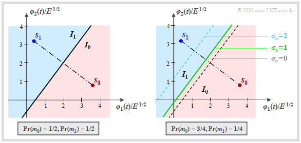
In the special case $N = 2$ and $M = 2$ considered here, the decision partitions the two-dimensional space into the two disjoint areas $I_0$ (highlighted in red) and $I_1$ (blue), as the graphic on the right illustrates.

If the received value lies in $I_0$, $m_0$ is output as the estimated value, otherwise $m_1$.

$\text{Derivation and picture description:}$ For the AWGN channel and $M = 2$, the decision rule is thus:

⇒ Always choose message $m_0$ if the following condition is satisfied:

$${\rm Pr}( m_0) \cdot {\rm exp} \left [ - \frac{1}{2 \sigma_n^2} \cdot \vert \hspace{-0.05cm} \vert \boldsymbol{ \rho } - \boldsymbol{ s }_0 \vert \hspace{-0.05cm} \vert^2 \right ] > {\rm Pr}( m_1) \cdot {\rm exp} \left [ - \frac{1}{2 \sigma_n^2} \cdot\vert \hspace{-0.05cm} \vert \boldsymbol{ \rho } - \boldsymbol{ s }_1 \vert \hspace{-0.05cm} \vert^2 \right ] \hspace{0.05cm}.$$

⇒ The boundary line between the two decision regions $I_0$ and $I_1$ is obtained by replacing the "greater sign" with the "equals sign" in the above equation and transforming the equation slightly:

$$\vert \hspace{-0.05cm} \vert \boldsymbol{ \rho } - \boldsymbol{ s }_0 \vert \hspace{-0.05cm} \vert^2 - 2 \sigma_n^2 \cdot {\rm ln} \hspace{0.15cm}\big [{\rm Pr}( m_0)\big ] = \vert \hspace{-0.05cm} \vert \boldsymbol{ \rho } - \boldsymbol{ s }_1 \vert \hspace{-0.05cm} \vert^2 - 2 \sigma_n^2 \cdot {\rm ln} \hspace{0.15cm}\big [{\rm Pr}( m_1)\big ]$$

$$\Rightarrow \hspace{0.3cm} \vert \hspace{-0.05cm} \vert \boldsymbol{ s }_1 \vert \hspace{-0.05cm} \vert^2 - \vert \hspace{-0.05cm} \vert \boldsymbol{ s }_0 \vert \hspace{-0.05cm} \vert^2 + 2 \sigma_n^2 \cdot {\rm ln} \hspace{0.15cm} \frac{ {\rm Pr}( m_0)}{ {\rm Pr}( m_1)} = 2 \cdot \boldsymbol{ \rho }^{\rm T} \cdot (\boldsymbol{ s }_1 - \boldsymbol{ s }_0)\hspace{0.05cm}.$$

From the plot above one can see:

The boundary curve between regions $I_0$ and $I_1$ is a straight line, since the equation of determination is linear in the received vector $\boldsymbol{ \rho } = (\rho_1, \hspace{0.05cm}\rho_2)$.

For equally probable symbols, the boundary is exactly halfway between $\boldsymbol{ s }_0$ and $\boldsymbol{ s }_1$ and rotated by $90^\circ$ with respect to the line connecting the transmission points:

$$\vert \hspace{-0.05cm} \vert \boldsymbol{ s }_1 \vert \hspace{-0.05cm} \vert ^2 - \vert \hspace{-0.05cm} \vert \boldsymbol{ s }_0 \vert \hspace{-0.05cm} \vert ^2 = 2 \cdot \boldsymbol{ \rho }^{\rm T} \cdot (\boldsymbol{ s }_1 - \boldsymbol{ s }_0)\hspace{0.05cm}.$$

For ${\rm Pr}(m_0) > {\rm Pr}(m_1)$, the decision boundary is shifted toward the less probable symbol $\boldsymbol{ s }_1$, and the more so the larger the AWGN standard deviation $\sigma_n$.

The green-dashed decision boundary in the right figure as well as the decision regions $I_0$ (red) and $I_1$ (blue) are valid for the (normalized) standard deviation $\sigma_n = 1$ and the dashed boundary lines for $\sigma_n = 0$ resp. $\sigma_n = 2$.

The special case of equally probable binary symbols

We continue to assume a binary system $(M = 2)$, but now consider the simple case where this can be described by a single basis function $(N = 1)$. The error probability for this has already been calculated in the section "Definition of the bit error probability".
With the nomenclature and representation form chosen for the fourth main chapter the following constellation results:

Conditional probability density functions for equally probable symbols

The received value $r = s + n$ is now a scalar and is composed of the transmitted signal $s \in \{s_0, \hspace{0.05cm}s_1\}$ and the noise term $n$ additively. The abscissa $\rho$ denotes a realization of $r$.

In addition, the abscissa is normalized to the reference quantity $\sqrt{E}$, whereas here the normalization energy $E$ has no prominent, physically interpretable meaning.

The noise term $n$ is Gaussian distributed with mean $m_n = 0$ and variance $\sigma_n^2$. The root of the variance $(\sigma_n)$ is called the "rms value" or the "standard deviation".

The decision boundary $G$ divides the entire value range of $r$ into the two subranges $I_0$ $($in which $s_0$ lies$)$ and $I_1$ $($with the signal value $s_1)$.

If $\rho > G$, the decision returns the estimated value $m_0$, otherwise $m_1$. It is assumed that the message $m_i$ is uniquely related to the signal $s_i$: $m_i \Leftrightarrow s_i$.

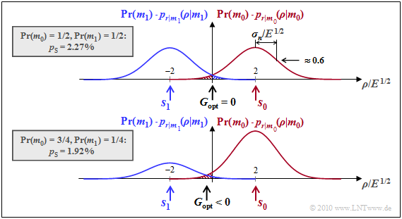
The graph shows the conditional $($one-dimensional$)$ probability density functions $p_{\hspace{0.02cm}r\hspace{0.05cm} \vert \hspace{0.05cm}m_0}$ and $p_{\hspace{0.02cm}r\hspace{0.05cm} \vert \hspace{0.05cm}m_1}$ for the AWGN channel, assuming equal symbol probabilities: ${\rm Pr}(m_0) = {\rm Pr}(m_1) = 0.5$. Thus, the $($optimal$)$ decision boundary is $G = 0$. One can see from this plot:

If $m = m_0$ and thus $s = s_0 = 2 \cdot E^{1/2}$, an erroneous decision occurs only if $\eta$, the realization of the noise quantity $n$, is smaller than $-2 \cdot E^{1/2}$.
In this case, $\rho < 0$, where $\rho$ denotes a realization of the received value $r$.
In contrast, for $m = m_1$ ⇒ $s = s_1 = -2 \cdot E^{1/2}$, an erroneous decision occurs whenever $\eta$ is greater than $+2 \cdot E^{1/2}$. In this case, $\rho > 0$.

Error probability for symbols with equal probability

Let ${\rm Pr}(m_0) = {\rm Pr}(m_1) = 0.5$. For AWGN noise with standard deviation $\sigma_n$, as already calculated in the section "Definition of the bit error probability" with different nomenclature, we obtain for the probability of a wrong decision $(\cal E)$ under the condition that message $m_0$ was sent:

$${\rm Pr}({ \cal E}\hspace{0.05cm} \vert \hspace{0.05cm} m_0) = \int_{-\infty}^{G = 0} p_{r \hspace{0.05cm}|\hspace{0.05cm}m_0 } ({ \rho } \hspace{0.05cm} \vert \hspace{0.05cm}m_0 ) \,{\rm d} \rho = \int_{-\infty}^{- s_0 } p_{{ n} \hspace{0.05cm}\vert\hspace{0.05cm}m_0 } ({ \eta } \hspace{0.05cm}|\hspace{0.05cm}m_0 ) \,{\rm d} \eta = \int_{-\infty}^{- s_0 } p_{{ n} } ({ \eta } ) \,{\rm d} \eta = \int_{ s_0 }^{\infty} p_{{ n} } ({ \eta } ) \,{\rm d} \eta = {\rm Q} \left ( {s_0 }/{\sigma_n} \right ) \hspace{0.05cm}.$$

In deriving the equation, it was considered that the AWGN noise $\eta$ is independent of the signal $(m_0$ or $m_1)$ and has a symmetric PDF. The complementary Gaussian error integral was also used:

$${\rm Q}(x) = \frac{1}{\sqrt{2\pi}} \int_{x}^{\infty} {\rm e}^{-u^2/2} \,{\rm d} u \hspace{0.05cm}.$$

Correspondingly, for $m = m_1$ ⇒ $s = s_1 = -2 \cdot E^{1/2}$:

$${\rm Pr}({ \cal E} \hspace{0.05cm}\vert\hspace{0.05cm} m_1) = \int_{0}^{\infty} p_{{ r} \hspace{0.05cm}\vert\hspace{0.05cm}m_1 } ({ \rho } \hspace{0.05cm}\vert\hspace{0.05cm}m_1 ) \,{\rm d} \rho = \int_{- s_1 }^{\infty} p_{{ n} } (\boldsymbol{ \eta } ) \,{\rm d} \eta = {\rm Q} \left ( {- s_1 }/{\sigma_n} \right ) \hspace{0.05cm}.$$

$\text{Conclusion:}$ With the distance $d = s_1 - s_0$ of the signal space points, we can summarize the results, still considering ${\rm Pr}(m_0) + {\rm Pr}(m_1) = 1$:

$${\rm Pr}({ \cal E}\hspace{0.05cm}\vert\hspace{0.05cm} m_0) = {\rm Pr}({ \cal E} \hspace{0.05cm}\vert\hspace{0.05cm} m_1) = {\rm Q} \big ( {d}/(2{\sigma_n}) \big )$$

$$\Rightarrow \hspace{0.3cm}{\rm Pr}({ \cal E} ) = {\rm Pr}(m_0) \cdot {\rm Pr}({ \cal E} \hspace{0.05cm}\vert\hspace{0.05cm} m_0) + {\rm Pr}(m_1) \cdot {\rm Pr}({ \cal E} \hspace{0.05cm}\vert\hspace{0.05cm} m_1)= \big [ {\rm Pr}(m_0) + {\rm Pr}(m_1) \big ] \cdot {\rm Q} \big [ {d}/(2{\sigma_n}) \big ] = {\rm Q} \big [ {d}/(2{\sigma_n}) \big ] \hspace{0.05cm}.$$

Notes:

This equation is valid under the condition $G = 0$ quite generally, thus also for ${\rm Pr}(m_0) \ne {\rm Pr}(m_1)$.
For "non-equally probable symbols", however, the error probability can be reduced by a different decision threshold.
The equation mentioned here is also valid if the signal space points are not scalars but are described by the vectors $\boldsymbol{ s}_0$ and $\boldsymbol{ s}_1$.
The distance $d$ results then as the norm of the difference vector: $d = \vert \hspace{-0.05cm} \vert \hspace{0.05cm} \boldsymbol{ s}_1 - \boldsymbol{ s}_0 \hspace{0.05cm} \vert \hspace{-0.05cm} \vert \hspace{0.05cm}.$

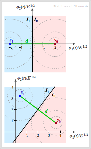
$\text{Example 1:}$ Let's look again at the signal space constellation from the "first chapter section" $($lower graphic$)$ with the values

Two signal space constellations

$\boldsymbol{ s}_0/E^{1/2} = (3.6, \hspace{0.05cm}0.8)$,

$\boldsymbol{ s}_1/E^{1/2} = (0.4, \hspace{0.05cm}3.2)$.

Here the distance of the signal space points is

$$d = \vert \hspace{-0.05cm} \vert s_1 - s_0 \vert \hspace{-0.05cm} \vert = \sqrt{E \cdot (0.4 - 3.6)^2 + E \cdot (3.2 - 0.8)^2} = 4 \cdot \sqrt {E}\hspace{0.05cm}.$$

This results in exactly the same value as for the upper constellation with

$\boldsymbol{ s}_0/E^{1/2} = (2, \hspace{0.05cm}0)$,

$\boldsymbol{ s}_1/E^{1/2} = (-2, \hspace{0.05cm}0)$.

The figures show these two constellations and reveal the following similarities and differences, assuming the AWGN noise variance $\sigma_n^2 = N_0/2$ in each case. The circles in the graph illustrate the circular symmetry of the two-dimensional AWGN noise.

As said before, both the distance of the signal points from the decision line $(d/2 = 2 \cdot \sqrt {E})$ and the AWGN characteristic value $\sigma_n$ are the same in both cases.

It follows: The two arrangements lead to the same error probability if the parameter $E$ $($a kind of normalization energy$)$ is kept constant:

$${\rm Pr} ({\rm symbol\hspace{0.15cm} error}) = {\rm Pr}({ \cal E} ) = {\rm Q} \big [ {d}/(2{\sigma_n}) \big ]\hspace{0.05cm}.$$

The "mean energy per symbol" $(E_{\rm S})$ for the upper constellation is given by

$$E_{\rm S} = 1/2 \cdot \vert \hspace{-0.05cm} \vert s_0 \vert \hspace{-0.05cm} \vert^2 + 1/2 \cdot \vert \hspace{-0.05cm} \vert s_1 \vert \hspace{-0.05cm} \vert^2 = E/2 \cdot \big[(+2)^2 + (-2)^2\big] = 4 \cdot {E}\hspace{0.05cm}.$$

With the lower constellation one receives in the same way:

$$E_{\rm S} = \ \text{...} \ = E/2 \cdot \big[(3.6)^2 + (0.8)^2\big] + E/2 \cdot \big[(0.4)^2 + (3.2)^2 \big] = 12 \cdot {E}\hspace{0.05cm}.$$

For a given mean energy per symbol ⇒ $E_{\rm S}$, the upper constellation is therefore clearly superior to the lower one: The same error probability results with one third of the energy per symbol. This issue will be discussed in detail in "Exercise 4.6Z".

Optimal threshold for non-equally probable symbols

If ${\rm Pr}(m_0) \ne {\rm Pr}(m_1)$ holds, a slightly smaller error probability can be obtained by shifting the decision threshold $G$. The following results are derived in detail in the solution to "Exercise 4.7":

For unequal symbol probabilities, the optimal decision threshold $G_{\rm opt}$ between regions $I_0$ and $I_1$ is closer to the less probable symbol. The normalized optimal shift with respect to the value $G = 0$ for equally probable symbols is

\[\gamma_{\rm opt} = \frac{G_{\rm opt}}{s_0 } = 2 \cdot \frac{ \sigma_n^2}{d^2} \cdot {\rm ln} \hspace{0.15cm} \frac{{\rm Pr}( m_1)}{{\rm Pr}( m_0)} \hspace{0.05cm}.\]

The error probability is then

$${\rm Pr}({ \cal E} ) = {\rm Pr}(m_0) \cdot {\rm Q} \big[ {d}/(2{\sigma_n}) \cdot (1 - \gamma_{\rm opt}) \big ] + {\rm Pr}(m_1) \cdot {\rm Q} \big [ {d}/(2{\sigma_n}) \cdot (1 + \gamma_{\rm opt}) \big ]\hspace{0.05cm}.$$

$\text{Example 2:}$ The formal parameter $\rho$ (abscissa) denotes a realization of the AWGN random variable $r = s + n$. For the following further holds:

Density functions for equal/unequal symbol probabilities

$$\boldsymbol{ s }_0 = (2 \cdot \sqrt{E}, \hspace{0.1cm} 0), \hspace{0.2cm} \boldsymbol{ s }_1 = (- 2 \cdot \sqrt{E}, \hspace{0.1cm} 0)$$

$$ \Rightarrow \hspace{0.2cm} d = 2 \cdot \sqrt{E}, \hspace{0.2cm} \sigma_n = \sqrt{E} \hspace{0.05cm}.$$

For equally probable symbols ⇒ ${\rm Pr}( m_0) = {\rm Pr}( m_1) = 1/2$, the optimal decision threshold is $G_{\rm opt} = 0$ ⇒ see upper sketch. This gives us for the error probability:

$${\rm Pr}({ \cal E} ) = {\rm Q} \big [ {d}/(2{\sigma_n}) \big ] = {\rm Q} (2) \approx 2.26\% \hspace{0.05cm}.$$

Now let the probabilities be ${\rm Pr}( m_0) = 3/4\hspace{0.05cm},\hspace{0.1cm}{\rm Pr}( m_1) = 1/4\hspace{0.05cm}$ ⇒ see lower sketch. Let the other system variables be unchanged from the upper graph. In this case the optimal (normalized) shift factor is

\[\gamma = 2 \cdot \frac{ \sigma_n^2}{d^2} \cdot {\rm ln} \hspace{0.15cm} \frac{ {\rm Pr}( m_1)}{ {\rm Pr}( m_0)} = 2 \cdot \frac{ E}{16 \cdot E} \cdot {\rm ln} \hspace{0.15cm} \frac{1/4}{3/4 } \approx - 0.14 \hspace{0.05cm}.\]

This is a $14\%$ shift toward the less probable symbol $\boldsymbol {s}_1$ (i.e., to the left). This makes the error probability slightly smaller than for equally probable symbols:

\[{\rm Pr}({ \cal E} )= 0.75 \cdot {\rm Q} \left ( 2 \cdot 1.14 \right ) + 0.25 \cdot {\rm Q} \left ( 2 \cdot 0.86 \right ) = 0.75 \cdot 0.0113 + 0.25 \cdot 0.0427 \approx 1.92\% \hspace{0.05cm}.\]

One recognizes from these numerical values:

Due to the threshold shift, the symbol $\boldsymbol {s}_1$ is now more distorted, but the more probable symbol $\boldsymbol {s}_0$ is distorted disproportionately less.
However, the result should not lead to misinterpretations. In the asymmetrical case ⇒ ${\rm Pr}( m_0) \ne {\rm Pr}( m_1)$ there is a smaller error probability than for ${\rm Pr}( m_0) ={\rm Pr}( m_1) = 0.5$, but then only less information can be transmitted with each symbol.
With the selected numerical values "$0.81 \ \rm bit/symbol$" instead of "$1\ \rm bit/symbol$".
From an information theoretic point of view, ${\rm Pr}( m_0) ={\rm Pr}( m_1)$ would be optimal.

$\text{Conclusion:}$

In the symmetric case ⇒ ${\rm Pr}( m_0) ={\rm Pr}( m_1)$, the conventional conditional PDF values $p_{r \hspace{0.05cm}\vert \hspace{0.05cm}m } ( \rho \hspace{0.05cm}\vert \hspace{0.05cm}m_i )$ can be used for decision.
In the asymmetric case ⇒ ${\rm Pr}( m_0) \ne {\rm Pr}( m_1)$, these functions must be weighted beforehand: ${\rm Pr}(m_i) \cdot p_{r \hspace{0.05cm}\vert \hspace{0.05cm}m_i } ( \rho \hspace{0.05cm}\vert \hspace{0.05cm}m_i )$.

In the following, we consider this issue.

Decision regions in the non-binary case

In general, the decision regions $I_i$ partition the $N$–dimensional real space into $M$ mutually disjoint regions.

Here, the decision region $I_i$ with $i = 0$, ... , $M-1$ is defined as the set of all points leading to the estimate $m_i$:

\[\boldsymbol{ \rho } \in I_i \hspace{0.2cm} \Leftrightarrow \hspace{0.2cm} \hat{m} = m_i, \hspace{0.3cm}{\rm where}\hspace{0.3cm}I_i = \left \{ \boldsymbol{ \rho } \in { \cal R}^N \hspace{0.05cm} | \hspace{0.05cm} {\rm Pr}( m_i) \cdot p_{\boldsymbol{ r} \hspace{0.05cm}|\hspace{0.05cm}m } (\boldsymbol{ \rho } \hspace{0.05cm} | \hspace{0.05cm} m_i ) > {\rm Pr}( m_k) \cdot p_{\boldsymbol{ r} \hspace{0.05cm}|\hspace{0.05cm}m } (\boldsymbol{ \rho } \hspace{0.05cm} | \hspace{0.05cm}m_k )\hspace{0.15cm} \forall k \ne i \right \} \hspace{0.05cm}.\]

The shape of the decision regions $I_i$ in the $N$–dimensional space depend on the conditional probability density functions $p_{r \hspace{0.05cm}\vert \hspace{0.05cm}m }$, i.e. on the considered channel.

In many cases – including the AWGN channel – the decision boundaries between every two signal points are straight lines, which simplifies further considerations.

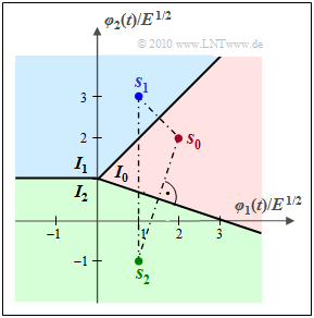
$\text{Example 3:}$ The graph shows the decision regions $I_0$, $I_1$ and $I_2$ for a transmission system with the parameters $N = 2$ and $M = 3$.

AWGN decision regions
$(N = 2$, $M = 3)$

The normalized transmission vectors here are

$$\boldsymbol{ s }_0 = (2,\hspace{0.05cm} 2),$$

$$ \boldsymbol{ s }_1 = (1,\hspace{0.05cm} 3),$$

$$ \boldsymbol{ s }_2 = (1,\hspace{0.05cm} -1) \hspace{0.05cm}.$$

Now two cases have to be distinguished:

For equally probable symbols ⇒ ${\rm Pr}( m_0) = {\rm Pr}( m_1) ={\rm Pr}( m_2) = 1/3 $, the boundaries between two regions are always straight, centered and perpendicular to the connecting lines.

In the case of unequal symbol probabilities, the decision boundaries are to be shifted $($parallel$)$ in the direction of the more improbable symbol in each case – the further the greater the AWGN standard deviation $\sigma_n$.

Error probability calculation in the non-binary case

After the decision regions $I_i$ are fixed, we can compute the symbol error probability of the overall system. We use the following names, although we sometimes have to use different names in continuous text than in equations because of the limitations imposed by our character set:

Symbol error probability: ${\rm Pr}({ \cal E} ) = {\rm Pr(symbol\hspace{0.15cm} error)} \hspace{0.05cm},$
Probability of correct decision: ${\rm Pr}({ \cal C} ) = 1 - {\rm Pr}({ \cal E} ) = {\rm Pr(correct \hspace{0.15cm} decision)} \hspace{0.05cm},$
Conditional probability of a correct decision under the condition $m = m_i$: ${\rm Pr}({ \cal C}\hspace{0.05cm}|\hspace{0.05cm} m_i ) = 1 - {\rm Pr}({ \cal E} \hspace{0.05cm}|\hspace{0.05cm} m_i) \hspace{0.05cm}.$

With these definitions, the probability of a correct decision is:

$${\rm Pr}({ \cal C} ) \hspace{-0.1cm} = \hspace{-0.1cm} \sum\limits_{i = 0}^{M-1} {\rm Pr}(m_i) \cdot {\rm Pr}({ \cal C}\hspace{0.05cm}|\hspace{0.05cm} m_i ) = \sum\limits_{i = 0}^{M-1} {\rm Pr}(m_i) \cdot {\rm Pr}(\boldsymbol{ r } \in I_i\hspace{0.05cm}|\hspace{0.05cm} m_i ) = \sum_{i = 0}^{M-1} {\rm Pr}(m_i) \cdot \int_{I_i} p_{{ \boldsymbol{ r }} \hspace{0.05cm}|\hspace{0.05cm}m } (\boldsymbol {\rho } \hspace{0.05cm}|\hspace{0.05cm} m_i ) \,{\rm d} \boldsymbol {\rho } \hspace{0.05cm}.$$

For the AWGN channel, this is according to the section "N–dimensional Gaussian noise":

\[{\rm Pr}({ \cal C}\hspace{0.05cm}|\hspace{0.05cm} m_i ) = 1 - {\rm Pr}({ \cal E} \hspace{0.05cm}|\hspace{0.05cm} m_i) = \frac{1}{(\sqrt{2\pi} \cdot \sigma_n)^N} \cdot \int_{I_i} {\rm exp} \left [ - \frac{1}{2 \sigma_n^2} \cdot || \boldsymbol{ \rho } - \boldsymbol{ s }_i ||^2 \right ] \,{\rm d} \boldsymbol {\rho }\hspace{0.05cm}.\]

This integral must be calculated numerically in the general case.
Only for a few, easily describable decision regions $\{I_i\}$ an analytical solution is possible.

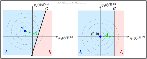
$\text{Example 4:}$ For the AWGN channel, there is a two-dimensional Gaussian bell around the transmission point $\boldsymbol{ s }_i$, recognizable in the left graphic by the concentric contour lines.

To calculate the error probability for AWGN

In addition, the decision line $G$ is drawn somewhat arbitrarily.
Shown alone on the right in a different coordinate system (shifted and rotated) is the PDF of the noise component.

The graph can be interpreted as follows:

The probability that the received vector does not fall into the blue "target area" $I_i$, but into the red highlighted area $I_k$, is $ {\rm Q} (A/\sigma_n)$; ${\rm Q}(x)$ is the Gaussian error function.

$A$ denotes the distance between $\boldsymbol{ s }_i$ and $G$. $\sigma_n$ indicates the "rms value" (root of the variance) of the AWGN noise.

Correspondingly, the probability for the event $r \in I_i$ is equal to the complementary value

\[{\rm Pr}({ \cal C}\hspace{0.05cm}\vert\hspace{0.05cm} m_i ) = {\rm Pr}(\boldsymbol{ r } \in I_i\hspace{0.05cm} \vert \hspace{0.05cm} m_i ) = 1 - {\rm Q} (A/\sigma_n)\hspace{0.05cm}.\]

We now consider the equations given above,

\[{\rm Pr}({ \cal C} ) = \sum\limits_{i = 0}^{M-1} {\rm Pr}(m_i) \cdot {\rm Pr}({ \cal C}\hspace{0.05cm}|\hspace{0.05cm} m_i ) \hspace{0.3cm}{\rm with} \hspace{0.3cm} {\rm Pr}({ \cal C}\hspace{0.05cm}|\hspace{0.05cm} m_i ) = \int_{I_i} p_{{ \boldsymbol{ r }} \hspace{0.05cm}|\hspace{0.05cm}m } (\boldsymbol {\rho } \hspace{0.05cm}|\hspace{0.05cm} m_i ) \,{\rm d} \boldsymbol {\rho } \hspace{0.05cm},\]

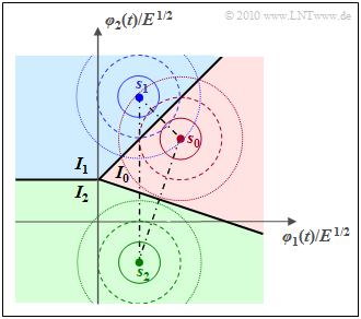
in a little more detail, where we again assume two basis functions $(N = 2)$ and three signal space points $(M = 3)$ at $\boldsymbol{ s }_0$, $\boldsymbol{ s }_1$, $\boldsymbol{ s }_2$.

Error probability calculation for AWGN, $M = 3$

The decision regions $I_0$, $I_1$ and $I_2$ are chosen "best as possible".
The AWGN noise is indicated in the sketch by three circular contour lines each.

One can see from this plot:

Assuming that $m = m_i \ \Leftrightarrow \ \boldsymbol{ s } = \boldsymbol{ s }_i$ was sent, a correct decision is made only if the received value $\boldsymbol{ r } \in I_i$.

The conditional probability ${\rm Pr}(\boldsymbol{ r } \in I_i\hspace{0.05cm}|\hspace{0.05cm}m_2)$ is (by far) largest for $i = 2$ ⇒ correct decision.

${\rm Pr}(\boldsymbol{ r } \in I_0\hspace{0.05cm}|\hspace{0.05cm}m_2)$ is much smaller. Almost negligible is ${\rm Pr}(\boldsymbol{ r } \in I_1\hspace{0.05cm}|\hspace{0.05cm}m_2)$.

Thus, the falsification probabilities for $m = m_0$ and $m = m_1$ are:

\[{\rm Pr}({ \cal E}\hspace{0.05cm}|\hspace{0.05cm} m_0 )={\rm Pr}(\boldsymbol{ r } \in I_1\hspace{0.05cm}|\hspace{0.05cm} m_0 ) + {\rm Pr}(\boldsymbol{ r } \in I_2\hspace{0.05cm}|\hspace{0.05cm} m_0 ),\]

\[ {\rm Pr}({ \cal E}\hspace{0.05cm}|\hspace{0.05cm} m_1 ) ={\rm Pr}(\boldsymbol{ r } \in I_0\hspace{0.05cm}|\hspace{0.05cm} m_1 ) + {\rm Pr}(\boldsymbol{ r } \in I_2\hspace{0.05cm}|\hspace{0.05cm} m_1 ) \hspace{0.05cm}.\]

The largest falsification probability is obtained for $m = m_0$. Because of

\[{\rm Pr}(\boldsymbol{ r } \in I_1\hspace{0.05cm}|\hspace{0.05cm} m_0 ) \approx {\rm Pr}(\boldsymbol{ r } \in I_0\hspace{0.05cm}|\hspace{0.05cm} m_1 ) \hspace{0.05cm}, \]

\[{\rm Pr}(\boldsymbol{ r } \in I_2\hspace{0.05cm}|\hspace{0.05cm} m_0 ) \gg {\rm Pr}(\boldsymbol{ r } \in I_2\hspace{0.05cm}|\hspace{0.05cm} m_1 ) \hspace{0.05cm}\]

the following relations hold:

$${\rm Pr}({ \cal E}\hspace{0.05cm}|\hspace{0.05cm} m_0 ) > {\rm Pr}({ \cal E}\hspace{0.05cm}|\hspace{0.05cm} m_1 ) >{\rm Pr}({ \cal E}\hspace{0.05cm}|\hspace{0.05cm} m_2 )\hspace{0.05cm}. $$

$\text{Conclusion:}$ These results can be summarized as follows:

To calculate the (average) error probability, it is necessary to average over all $M$ terms in general, even in the case of equally probable symbols.
In the case of equally probable symbols, ${\rm Pr}(m_i) = 1/M$ can be drawn in front of the summation, but this does not simplify the calculation very much.
Only in the case of symmetrical arrangement the averaging can be omitted.

Union Bound - Upper bound for the error probability

For arbitrary values of $M$, the following applies to the falsification probability under the condition that the message $m_i$ $($or the signal $\boldsymbol{s}_i)$ has been sent:

\[{\rm Pr}({ \cal E}\hspace{0.05cm}|\hspace{0.05cm} m_i ) = {\rm Pr} \left [ \bigcup_{k \ne i} { \cal E}_{ik}\right ] \hspace{0.05cm},\hspace{0.5cm}{ \cal E}_{ik}\hspace{-0.1cm}: \boldsymbol{ r }{\rm \hspace{0.15cm}is \hspace{0.15cm}closer \hspace{0.15cm}to \hspace{0.15cm}}\boldsymbol{ s }_k {\rm \hspace{0.15cm}than \hspace{0.15cm}to \hspace{0.15cm}the \hspace{0.15cm}nominal \hspace{0.15cm}value \hspace{0.15cm}}\boldsymbol{ s }_i \hspace{0.05cm}. \]

$\text{Definition:}$ An upper bound can be specified for this expression with a Boolean inequality – the so-called Union Bound:

\[{\rm Pr}({ \cal E}\hspace{0.05cm}\vert\hspace{0.05cm} m_i ) \le \sum\limits_{k = 0, \hspace{0.1cm}k \ne i}^{M-1} {\rm Pr}({ \cal E}_{ik}) = \sum\limits_{k = 0, \hspace{0.1cm}k \ne i}^{M-1}{\rm Q} \big [ d_{ik}/(2{\sigma_n}) \big ]\hspace{0.05cm}. \]

Remarks:

$d_{ik} = \vert \hspace{-0.05cm} \vert \boldsymbol{s}_i - \boldsymbol{s}_k \vert \hspace{-0.05cm} \vert$ is the distance between the signal space points $\boldsymbol{s}_i$ and $\boldsymbol{s}_k$.
$\sigma_n$ specifies the rms value of the AWGN noise.
The "Union Bound" can only be used for equally probable symbols ⇒ ${\rm Pr}(m_i) = 1/M$.
But also in this case, an average must be taken over all $m_i$ in order to calculate the (average) error probability.

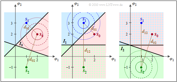
$\text{Example 5:}$ The graphic illustrates the Union Bound using the example of $M = 3$ with equally probable symbols: ${\rm Pr}(m_0) = {\rm Pr}(m_1) = {\rm Pr}(m_2) =1/3$.

To clarify the "Union Bound"

The following should be noted about these representations:

The following applies to the symbol error probability:

$${\rm Pr}({ \cal E} ) = 1 - {\rm Pr}({ \cal C} ) \hspace{0.05cm},$$

$${\rm Pr}({ \cal C} ) = {1}/{3} \cdot \big [ {\rm Pr}({ \cal C}\hspace{0.05cm}\vert \hspace{0.05cm} m_0 ) + {\rm Pr}({ \cal C}\hspace{0.05cm}\vert \hspace{0.05cm} m_1 ) + {\rm Pr}({ \cal C}\hspace{0.05cm}\vert \hspace{0.05cm} m_2 ) \big ]\hspace{0.05cm}.$$

The first term ${\rm Pr}(\boldsymbol{r} \in I_0\hspace{0.05cm}\vert \hspace{0.05cm} m_0)$ in the expression in brackets under the assumption $m = m_0 \ \Leftrightarrow \ \boldsymbol{s} = \boldsymbol{s}_0$ is visualized in the left graphic by the red region $I_0$.

The complementary region ${\rm Pr}(\boldsymbol{r} \not\in I_0\hspace{0.05cm}\vert \hspace{0.05cm} m_0)$ is marked on the left with either blue or green or blue–green hatching. It applies ${\rm Pr}({ \cal C}\hspace{0.05cm}\vert\hspace{0.05cm} m_0 ) = 1 - {\rm Pr}({ \cal E}\hspace{0.05cm}\vert \hspace{0.05cm} m_0 )$ with

$${\rm Pr}({ \cal E}\hspace{0.05cm}\vert\hspace{0.05cm} m_0 ) = {\rm Pr}(\boldsymbol{ r } \in I_1 \hspace{0.05cm}\cup \hspace{0.05cm} \boldsymbol{ r } \in I_2 \hspace{0.05cm}\vert\hspace{0.05cm} m_0 ) $$

$$\Rightarrow \hspace{0.3cm} {\rm Pr}({ \cal E}\hspace{0.05cm}\vert\hspace{0.05cm} m_0 ) \le {\rm Pr}(\boldsymbol{ r } \in I_1 \hspace{0.05cm}\vert\hspace{0.05cm} m_0 ) + {\rm Pr}(\boldsymbol{ r } \in I_2 \hspace{0.05cm}\vert\hspace{0.05cm} m_0 ) $$

$$\Rightarrow \hspace{0.3cm} {\rm Pr}({ \cal E}\hspace{0.05cm}\vert\hspace{0.05cm} m_0 ) \le {\rm Q} \big [ d_{01}/(2{\sigma_n}) \big ]+ {\rm Q} \big [ d_{02}/(2{\sigma_n}) \big ] \hspace{0.05cm}.$$

The "less/equal" sign takes into account that the blue–green hatched area belongs both to the area "$\boldsymbol{r} \in I_1$" and to the area "$\boldsymbol{r} \in I_2$", so that the sum returns a value that is too large. This means: The Union Bound always provides an upper bound.

The middle graph illustrates the calculation under the assumption that $m = m_1 \ \Leftrightarrow \ \boldsymbol{s} = \boldsymbol{s}_1$ was sent. The figure on the right is based on $m = m_2 \ \Leftrightarrow \ \boldsymbol{s} = \boldsymbol{s}_2$.

Further effort reduction at Union Bound

The estimation according to the "Union Bound" can be further improved by considering only those signal space points that are direct neighbors of the current transmitted vector $\boldsymbol{s}_i$:

Definition of the neighboring sets $N(i)$

\[{\rm Pr}({ \cal E}\hspace{0.05cm}|\hspace{0.05cm} m_i ) = \sum\limits_{k = 0, \hspace{0.1cm} k \ne i}^{M-1}{\rm Q}\big [ d_{ik}/(2{\sigma_n}) \big ] \hspace{0.2cm} \Rightarrow \hspace{0.2cm} {\rm Pr}({ \cal E}\hspace{0.05cm}|\hspace{0.05cm} m_i ) = \sum\limits_{k = 0, \hspace{0.1cm} k \hspace{0.05cm}\in \hspace{0.05cm}N(i)}^{M-1}\hspace{-0.4cm}{\rm Q} \big [ d_{ik}/(2{\sigma_n}) \big ] \hspace{0.05cm}. \]

To do this, we define the "neighbors" of $\boldsymbol{s}_i$ as

\[N(i) = \big \{ k \in \left \{ i = 0, 1, 2, \hspace{0.05cm}\text{...} \hspace{0.05cm}, M-1 \big \}\hspace{0.05cm}|\hspace{0.05cm} I_i {\rm \hspace{0.15cm}is \hspace{0.15cm}directly \hspace{0.15cm}adjacent \hspace{0.15cm}to \hspace{0.15cm}}I_k \right \} \hspace{0.05cm}. \]

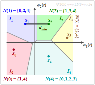
The graphic illustrates this definition using $M = 5$ as an example.

Regions $I_0$ and $I_3$ each have only two direct neighbors,
while $I_4$ borders all other decision regions.

The introduction of the neighboring sets $N(i)$ improves the quality of the Union Bound approximation, which means that the limit is then closer to the actual error probability, i.e. it is shifted down.

Another and frequently used limit uses only the minimum distance $d_{\rm min}$ between two signal space points.

In the above example, this occurs between $\boldsymbol{s}_1$ and $\boldsymbol{s}_2$.

For equally probable symbols ⇒ ${\rm Pr}(m_i) =1/M$ the following estimation then applies:

\[{\rm Pr}({ \cal E} ) \le \sum\limits_{i = 0 }^{M-1} \left [ {\rm Pr}(m_i) \cdot \sum\limits_{k \ne i }{\rm Q} \big [d_{ik}/(2{\sigma_n})\big ] \right ] \le \frac{1}{M} \cdot \sum\limits_{i = 0 }^{M-1} \left [ \sum\limits_{k \ne i } {\rm Q} [d_{\rm min}/(2{\sigma_n})] \right ] = \sum\limits_{k \ne i }{\rm Q} \big [d_{\rm min}/(2{\sigma_n})\big ] = (M-1) \cdot {\rm Q} \big [d_{\rm min}/(2{\sigma_n})\big ] \hspace{0.05cm}. \]

It should be noted here:

This limit is also very easy to calculate for large $M$ values. In many applications, however, this results in a much too high value for the error probability.
The limit is equal to the actual error probability if all regions are directly adjacent to all others and the distances of all $M$ signal points from one another are $d_{\rm min}$.
In the special case $M = 2$, these two conditions are often met, so that the "Union Bound" corresponds exactly to the actual error probability.