Difference between revisions of "Digital Signal Transmission/Decision Feedback"
| (26 intermediate revisions by 5 users not shown) | |||
| Line 1: | Line 1: | ||
{{Header | {{Header | ||
| − | |Untermenü= | + | |Untermenü=Intersymbol Interfering and Equalization Methods |
|Vorherige Seite=Lineare Nyquistentzerrung | |Vorherige Seite=Lineare Nyquistentzerrung | ||
|Nächste Seite=Optimale Empfängerstrategien | |Nächste Seite=Optimale Empfängerstrategien | ||
}} | }} | ||
| − | == | + | == Principle and block diagram == |
<br> | <br> | ||
| − | + | {{BlaueBox|TEXT= | |
| + | $\text{Definition:}$ '''Decision Feedback Equalization''' $\rm (DFE)$ is a method of reducing intersymbol interference. In German-language literature, this is sometimes also referred to as "Quantized Feedback" $\rm (QR)$.}} | ||
| − | |||
| − | |||
| − | |||
| − | |||
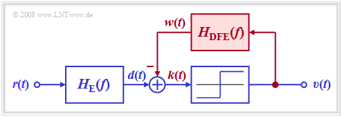
| − | + | The graphic shows the corresponding receiver. It can be seen from the block diagram: | |
| − | + | [[File:P ID1446 Dig T 3 6 S1 version1.png|right|frame|Receiver with decision feedback equalization $\rm (DFE)$|class=fit]] | |
| − | |||
| − | |||
| − | |||
| + | *Without the signal feedback shown in red, a conventional digital receiver with threshold decision would result according to the chapter [[Digital_Signal_Transmission/Consideration_of_Channel_Distortion_and_Equalization#Ideal_channel_equalizer|"Ideal channel equalizer"]]. | ||
| + | |||
| + | *For the following description, it is assumed that the entire receiver filter $H_{\rm E}(f)$ is composed of the (fictitious) ideal channel equalizer $1/H_{\rm K}(f)$ and a Gaussian low-pass filter $H_{\rm G}(f)$ for noise power limitation. | ||
| − | + | *In the receiver with decision feedback, a compensation signal $w(t)$ is obtained from the rectangular output signal $v(t)$ via a linear network with the frequency response $H_{\rm DFE}(f)$ and fed back to the input of the threshold decision.<br> | |
| − | ''' | + | *This signal $w(t)$ is subtracted from the pre-equalized signal $d(t)$. If the feedback network is suitably dimensioned, the '''corrected signal''' $k(t) = d(t) - w(t)$ thus has no (or at least significantly fewer) pulse trailers than the signal $d(t)$. |
| − | + | *In contrast to these pulse trailers ("postcursors"), the pulse precursors cannot be influenced for reasons of causality. | |
| − | + | *Since in this receiver with decision feedback, the compensation signal $w(t)$ is derived from the noise-free sink signal $v(t)$, the signal equalization is not associated with an increase in noise power as in linear equalization. Rather, the corrected signal $k(t)$ has the same noise rms value $\sigma_d$ as the signal $d(t)$.<br><br> | |
| − | : | + | ⇒ The signal characteristics of this nonlinear equalization method "DFE" as well as the associated error probabilities – valid for a distortion-free channel – can be displayed with the (German language) SWF applet [[Applets:Entscheidungsrückkopplung|"Entscheidungsrückkopplung"]] ⇒ "Decision Feedback Equalization" |
| − | |||
| − | |||
| − | == | + | == Ideal decision feedback == |
<br> | <br> | ||
| − | + | We first discuss the ideal DFE realization based on the different basic pulses.<br> | |
{{BlaueBox|TEXT= | {{BlaueBox|TEXT= | ||
| − | $\text{Definition:}$ | + | $\text{Definition:}$ An '''ideal decision feedback''' exists when the following basic pulse is applied to the decision: |
:$$g_k(t) = \left\{ \begin{array}{c} g_d(t) | :$$g_k(t) = \left\{ \begin{array}{c} g_d(t) | ||
\\ 0 \\ \end{array} \right.\quad | \\ 0 \\ \end{array} \right.\quad | ||
| − | \begin{array}{*{1}c} \text{ | + | \begin{array}{*{1}c} \text{for} \\ \text{for} \\ \end{array} |
\begin{array}{*{20}c} t < T_{\rm D} + T_{\rm V}, \\ t \ge T_{\rm D} + T_{\rm V}. \\ | \begin{array}{*{20}c} t < T_{\rm D} + T_{\rm V}, \\ t \ge T_{\rm D} + T_{\rm V}. \\ | ||
| − | \end{array}$$ | + | \end{array}$$ |
| + | *This means that in the ideal case the basic compensation pulse $g_w(t)$ must exactly reproduce the linearly pre-equalized pulse $g_d(t)$ for all times $t > T_{\rm D} + T_{\rm V}$. | ||
| + | |||
| + | *The delay time $T_{\rm V}$ required for realization reasons must be smaller than the symbol duration $T$; In the following $T_{\rm V} = T/2$ always applies.}}<br> | ||
| − | + | {{GraueBox|TEXT= | |
| + | $\text{Example 1:}$ Let the total frequency response $H_{\rm K}(f) \cdot H_{\rm E}(f) = H_{\rm G}(f)$ be Gaussian with the cutoff frequency $f_{\rm G} = 0.3/T$. For NRZ rectangular pulses, this then yields the basic pulse $g_d(t)$ sketched in pink. | ||
| − | + | [[File:P ID1447 Dig T 3 6 S2 version1.png|right|frame|Basic pulses and signals with ideal "Decision Feedback Equalization" $\rm (DFE)$|class=fit]] | |
| − | |||
| − | + | ⇒ Shown on the left are the basic pulses $g_w(t)$ and $g_k(t)$ with ideal decision feedback, based on the detection time $T_{\rm D} = 0$ and the delay time $T_{\rm V} = T/2$. <br> | |
| − | [ | + | ⇒ The right pictures from [Söd01]<ref name = 'Söd01'>Söder, G.: Simulation digitaler Übertragungssysteme. Anleitung zum gleichnamigen Praktikum. Lehrstuhl für Nachrichtentechnik, Technische Universität München, 2001.</ref> – all without consideration of the noise – make clear that by the compensation of all pulse trailers by means of the correction signal $w(t)$, the distances of the useful signal samples $d_{\rm S}(\nu \cdot T)$ from the decision threshold $E = 0$ are changed. |
| − | + | *Particularly small distances, such as at times $t = 6T$ and $t = 7T$, are significantly increased and thus their error probabilities are greatly reduced (arrows pointing away from the threshold).<br> | |
| − | |||
| − | * | + | *In contrast, the samples further away from the threshold value $E = 0$ in the signal $d(t)$ are shifted towards the threshold and their falsification probabilities are thus slightly increased. This can be seen, for example, for time $t = 5T$.}}<br> |
| − | == | + | == Eye opening and error probability with DFE == |
<br> | <br> | ||
| − | + | [[File:EN_Dig_T_3_6_S3.png|right|frame|Eye diagrams without and with "Decision Feedback Equalization" $(f_{\rm G}\cdot T = 0.3)$|class=fit]] We now consider the eye diagrams | |
| − | :$$g_0 = g_d(t=0) = 0.548 \cdot s_0 | + | *without DFE (left graph) and |
| − | + | *with ideal DFE (right graph). | |
| − | g_{-1} \hspace{0.05cm}, | + | |
| − | \hspace{0.05cm}, | + | |
| + | We assume the same conditions as in the last section, so that the following basic pulse values are present: | ||
| + | :$$g_0 = g_d(t=0) = 0.548 \cdot s_0,$$ | ||
| + | :$$g_1 = g_d(t=T) = 0.214 \cdot s_0 = | ||
| + | g_{-1} \hspace{0.05cm},$$ | ||
| + | :$$g_2 = g_d(t=2\hspace{0.05cm}T) = 0.012 \cdot s_0 = g_{-2} | ||
| + | \hspace{0.05cm},$$ | ||
| + | :$$g_3 = g_{-3} = \text{...} \approx 0 | ||
\hspace{0.05cm}.$$ | \hspace{0.05cm}.$$ | ||
| − | + | These two eye diagrams can be interpreted as follows: | |
| − | + | *For the conventional receiver (without DFE), with binary bipolar redundancy-free coding considering symmetry: | |
| − | |||
| − | * | ||
:$${\ddot{o}(T_{\rm D} = 0 )} = {2} \cdot \big [ g_0 - | g_{-1}| - | g_{-2}| - | g_{1}| - | g_{2}|\big ] = {2} \cdot \big [ g_0 - 2 \cdot g_{1} - 2 \cdot g_{2}\big | :$${\ddot{o}(T_{\rm D} = 0 )} = {2} \cdot \big [ g_0 - | g_{-1}| - | g_{-2}| - | g_{1}| - | g_{2}|\big ] = {2} \cdot \big [ g_0 - 2 \cdot g_{1} - 2 \cdot g_{2}\big | ||
]= 0.192 \cdot s_0 \hspace{0.05cm}.$$ | ]= 0.192 \cdot s_0 \hspace{0.05cm}.$$ | ||
| − | * | + | *On the other hand, for ideal DFE, the two trailers $g_1$ and $g_2$ are fully compensated and we obtain for the vertical eye opening: |
:$${\ddot{o}(T_{\rm D} = 0 )} = {2} \cdot \big [ g_0 - | g_{-1}| - |g_{-2}|\big | :$${\ddot{o}(T_{\rm D} = 0 )} = {2} \cdot \big [ g_0 - | g_{-1}| - |g_{-2}|\big | ||
] = {2} \cdot \big [ g_0 - g_{1} - g_{2}\big ]= 0.644 \cdot s_0 \hspace{0.05cm}.$$ | ] = {2} \cdot \big [ g_0 - g_{1} - g_{2}\big ]= 0.644 \cdot s_0 \hspace{0.05cm}.$$ | ||
| − | * | + | *Since the correction signal $w(t)$ is derived from the decision and thus noise-free signal $v(t)$, the noise rms value $\sigma_d$ is not changed by the decision feedback. Thus, the SNR gain due to the DFE is |
:$$G_{\rm DFE}= | :$$G_{\rm DFE}= | ||
20 \cdot {\rm lg}\hspace{0.1cm}\frac{0.644}{0.192} \approx 10.5\,{\rm dB} \hspace{0.05cm}.$$ | 20 \cdot {\rm lg}\hspace{0.1cm}\frac{0.644}{0.192} \approx 10.5\,{\rm dB} \hspace{0.05cm}.$$ | ||
{{BlaueBox|TEXT= | {{BlaueBox|TEXT= | ||
| − | $\text{ | + | $\text{Conclusion:}$ For a coaxial cable with characteristic cable attenuation $a_\star = 80 \ \rm dB$ and $10 \cdot \lg \ (E_{\rm B}/N_0) = 80 \ \rm dB$, <br>this SNR gain means that the worst-case error probability $p_{\rm U}$ is reduced by DFE from $7\%$ to about $4 \cdot 10^{-7}$ – a quite remarkable improvement.}}<br> |
| − | == | + | == Optimization of a transmission system with DFE == |
<br> | <br> | ||
| − | [[File: | + | |
| − | + | The last section has already made clear that the DFE already causes an enormous SNR gain if | |
| − | * | + | [[File:EN_Dig_T_3_6_S3_v23png.png|right|frame|Eye diagrams with DFE and optimized detection time|class=fit]] |
| − | * | + | * a fixed cutoff frequency $f_{\rm G}$ and |
| + | *the fixed detection time $T_{\rm D} = 0$ | ||
| − | + | is assumed. However, the system can be further improved if the two parameters $f_{\rm G}$ and $T_{\rm D}$ are optimized together.<br> | |
| − | + | The graph shows the eye diagrams without noise for | |
| − | *$f_{\rm G} \cdot T = 0.3$ ( | + | *$f_{\rm G} \cdot T = 0.3$ (left), |
| − | *$f_{\rm G} \cdot T = 0.2$ ( | + | *$f_{\rm G} \cdot T = 0.2$ (right). |
| − | + | For the diagram and the following calculations are still assumed: | |
| + | *the characteristic cable attenuation $a_\star = 80 \ \rm dB$, | ||
| + | *the AWGN parameter $10 \cdot \lg \ (E_{\rm B}/N_0) = 80 \ \rm dB$ <br>$($with $E_{\rm B} = s_0^2 \cdot T)$. | ||
| − | |||
| + | The left diagram is largely identical – except for the detection time $T_{\rm D}$ – to the [[Digital_Signal_Transmission/Decision_Feedback#Eye_opening_and_error_probability_with_DFE|right diagram]] in the last section. The optimization results can be summarized as follows: | ||
| − | + | *With $f_{\rm G} \cdot T = 0.3$, by shifting the detection time to $T_\text{D, opt} = -0.3T$, the eye opening can be increased to $\ddot{o}(T_\text{D, opt}) = 0.779 \cdot s_0 $. | |
| + | |||
| + | *Compared to $T_{\rm D} = 0$ $($see last section$)$, this results in a further SNR gain of $G_{T_\text{D, opt}}= 20 \cdot {\rm lg}\hspace{0.1cm}{0.779}/{644} \approx 1.65\,{\rm dB} \hspace{0.05cm}.$ | ||
| + | |||
| + | *The worst-case error probability is now found to be $p_{\rm U} \approx 1.3 \cdot 10^{-9}$ $($versus $4 \cdot 10^{-7})$.<br> | ||
| − | |||
| − | |||
| − | |||
| + | With the DFE receiver, however, you can further reduce the cutoff frequency. The reason is the better noise behavior with a smaller cutoff frequency. | ||
| + | *For example, the normalized noise rms value results instead of $\sigma_d/s_0 = 0.065$ $($for $f_{\rm G} \cdot T = 0.3)$ to $\sigma_d/s_0 = 0.010$ $($for $f_{\rm G} \cdot T = 0.2)$. | ||
| − | + | *Thus, with $f_{\rm G} \cdot T = 0.2$ and $T_{\rm D} = 0$ the small but nonzero eye opening $\ddot{o}_{\rm norm} = 0.152$ is obtained, which together with the very favorable noise rms value leads to the worst-case SNR $10 \cdot \lg \ \rho_{\rm U} = 17.6 \ \rm dB$ ⇒ worst-case error probabilty $p_{\rm U} \approx 1.6 \cdot 10^{-14}$. | |
| − | + | ||
| − | * | + | *By combining the cutoff frequency $f_{\rm G} \cdot T = 0.2$ with the detection time $T_{\rm D} = -T/2$, one finally obtains the optimal system configuration with the normalized eye opening $\ddot{o}_{\rm norm} = 0.368$ and the worst-case SNR $10 \cdot \lg \ \rho_{\rm U} = 25.3 \ \rm dB$. |
| − | |||
| + | * Thus (practically) $p_{\rm U}\approx 0$. However, this configuration is not relevant in practice: Already a minimal tolerance of the system parameters leads to a "closed eye".<br> | ||
| − | == | + | |
| + | == Realization aspects of the decision feedback == | ||
<br> | <br> | ||
| − | + | As an essential result of the last chapter [[Digital_Signal_Transmission/Linear_Nyquist_Equalization|"Linear Nyquist Equalization"]] and the current chapter "Decision Feedback" the following approach is recommended: | |
{{BlaueBox|TEXT= | {{BlaueBox|TEXT= | ||
| − | $\text{ | + | $\text{Conclusion:}$ For a transmission system over copper lines $($coaxial cable, two-wire line$)$, the following system variants are particularly suitable due to the achievable signal–to–noise ratio at the decision: |
| − | * | + | *a '''multi-level system''' $($for example $M = 4)$ and the optimal '''Nyquist equalization''' to compensate for the strong intersymbol interference caused by the linear channel distortions;<br> |
| − | * | + | |
| + | *a '''binary system''' with relatively small bandwidth of the total frequency response $H_{\rm G}(f) = H_{\rm K}(f) \cdot H_{\rm E}(f)$ and a non-linear decision with '''DFE'''.}} | ||
| − | + | Both system variants provide comparably good results under idealized conditions. But it should be noted, that large degradations can occur due to realization inaccuracies in both systems, which are mentioned here using the DFE system as an example: | |
| − | * | + | *Since no DC signal can be transmitted via the telephone network, but $H_{\rm K}(f=0) = 1$ is assumed for our calculations, a "DC signal recovery" is required at the receiver. This statement applies in the same way to the quaternary Nyquist system.<br> |
| − | * | + | *In the DFE system, the compensation pulse $g_w(t)$ must exactly replicate the pre-equalized basic pulse $g_d(t)$. This is especially difficult when $g_d(t)$ is very broad $($small cutoff frequency, e.g. $f_{\rm G} \cdot T = 0.2)$ and the optimization yields the detection time $T_\text{D, opt} = -T/2$.<br> |
| − | * | + | *If a wrong decision occurs due to a large noise value, the subsequent symbols will also be falsified with a high probability. However, there are always symbol sequences which interrupt this [https://en.wikipedia.org/wiki/Propagation_of_uncertainty "propogation of uncertainty"]. <br> |
| − | {{GraueBox|TEXT= | + | {{GraueBox|TEXT= |
| − | $\text{ | + | [[File:EN_Dig_T_3_6_S5a.png|right|frame|Basic pulses with ideal DFE|class=fit]] |
| + | $\text{Example 2:}$ The graph shows the basic pulse $g_d(t)$ | ||
| + | * for the cutoff frequency $f_{\rm G} \cdot T = 0.2$ (red curve) and | ||
| + | * the compensation pulse $g_w(t)$ for $T_\text{D} = -T/2$ (filled in blue). | ||
| − | |||
| − | * | + | Here, a delay time $T_\text{V} = -T/2$ between decision and start of signal correction is considered. It can be seen: |
| − | * | + | *For $T_\text{D} = -T/2$ the first trailer $g_d(T_\text{D} +T) = g_d(T/2)$ is exactly as large as the main value $g_d(T_\text{D}) = g_d(-T/2)$. |
| + | |||
| + | *If it is not possible to fully compensate all the trailers, this quickly results in a closed eye and thus, in the worst–case error probability $p_{\rm U} \approx 50\%$.}}<br> | ||
| − | == | + | == Decision feedback with delay filter== |
<br> | <br> | ||
| − | [[File:P ID1451 Dig T 3 6 S5b version1.png|right|frame| | + | For a circuit realization it is sufficient if the basic corrected pulse $g_k(t)$ becomes zero only at the equidistant detection times $T_\text{D} +\nu \cdot T$. |
| − | + | [[File:P ID1451 Dig T 3 6 S5b version1.png|right|frame|Decision feedback with delay filter|class=fit]] | |
| + | One realization possibility is thus an asymmetric [[Digital_Signal_Transmission/Linear_Nyquist_Equalization#Operating_principle_of_the_transversal_filter|delay filter]] according to the adjacent diagram, | ||
| − | + | *whose order $N$ (number of filter coefficients), and<br> | |
| − | * | + | *whose filter coefficients $ k_\nu$ $($mit $\nu = 1$, ... , $N)$ |
| − | |||
| − | |||
| + | are determined by the pulse $g_d(t)$ and the detection time $T_\text{D}$. <br> | ||
| − | |||
| − | |||
| − | * | + | This DFE realization has the following properties: |
| + | *Since the output signal $v(t)$ is rectangular, the compensation pulse $g_w(t)$ is staircase shaped.<br> | ||
| + | |||
| + | *With proper dimensioning of the filter coefficients $k_\nu$, <br>for $\nu = 1$, ... , $N$: | ||
:$$g_w(T_{\rm D} + \nu \cdot T) = g_d(T_{\rm D} + \nu \cdot T) | :$$g_w(T_{\rm D} + \nu \cdot T) = g_d(T_{\rm D} + \nu \cdot T) | ||
\hspace{0.3cm}\Rightarrow\hspace{0.3cm} | \hspace{0.3cm}\Rightarrow\hspace{0.3cm} | ||
g_k(T_{\rm D} + \nu \cdot T) = 0 \hspace{0.05cm}.$$ | g_k(T_{\rm D} + \nu \cdot T) = 0 \hspace{0.05cm}.$$ | ||
| − | * | + | *At detection time $T_\text{D}$, the vertical eye opening is exactly the same as for ideal DFE. A disadvantage is a smaller horizontal eye opening.<br><br> |
| − | {{GraueBox|TEXT= | + | {{GraueBox|TEXT= |
| − | $\text{ | + | [[File:P ID1452 Dig T 3 6 S5c version1.png|right|frame|Basic pulses for DFE with delay filter|class=fit]] |
| + | |||
| + | $\text{Example 3:}$ The graph shows the basic pulses $g_d(t)$ and $g_w(t)$ for decision feedback with a second order delay filter. The same conditions apply as for the example in the last section: $f_{\rm G} \cdot T = 0.2$ and $T_\text{D} = -T/2$. One can see: | ||
| − | + | *Because of the order $N = 2$, only the first two trailers $g_d(0.5T)$ and $g_d(1.5T)$ are compensated here. | |
| − | * | + | *The third trailer $g_d(2.5T)$ could be compensate by a further filter coefficient $k_3$. |
| − | + | ||
| − | * | + | *In contrast, the precursors $g_d(-1.5T)$ and $g_d(-2.5T)$ cannot be compensated in principle.}}<br> |
| − | == | + | ==Exercises for the chapter== |
<br> | <br> | ||
| − | [[Aufgaben: | + | [[Aufgaben:Exercise_3.8:_Delay_Filter_DFE_Realization|Exercise 3.8: Delay Filter DFE Realization]] |
| − | [[Aufgaben: | + | [[Aufgaben:Exercise_3.8Z:_Optimal_Detection_Time_for_DFE|Exercise 3.8Z: Optimal Detection Time for DFE]] |
| − | == | + | ==References== |
<references/> | <references/> | ||
Latest revision as of 17:26, 24 August 2022
Contents
Principle and block diagram
$\text{Definition:}$ Decision Feedback Equalization $\rm (DFE)$ is a method of reducing intersymbol interference. In German-language literature, this is sometimes also referred to as "Quantized Feedback" $\rm (QR)$.
The graphic shows the corresponding receiver. It can be seen from the block diagram:
- Without the signal feedback shown in red, a conventional digital receiver with threshold decision would result according to the chapter "Ideal channel equalizer".
- For the following description, it is assumed that the entire receiver filter $H_{\rm E}(f)$ is composed of the (fictitious) ideal channel equalizer $1/H_{\rm K}(f)$ and a Gaussian low-pass filter $H_{\rm G}(f)$ for noise power limitation.
- In the receiver with decision feedback, a compensation signal $w(t)$ is obtained from the rectangular output signal $v(t)$ via a linear network with the frequency response $H_{\rm DFE}(f)$ and fed back to the input of the threshold decision.
- This signal $w(t)$ is subtracted from the pre-equalized signal $d(t)$. If the feedback network is suitably dimensioned, the corrected signal $k(t) = d(t) - w(t)$ thus has no (or at least significantly fewer) pulse trailers than the signal $d(t)$.
- In contrast to these pulse trailers ("postcursors"), the pulse precursors cannot be influenced for reasons of causality.
- Since in this receiver with decision feedback, the compensation signal $w(t)$ is derived from the noise-free sink signal $v(t)$, the signal equalization is not associated with an increase in noise power as in linear equalization. Rather, the corrected signal $k(t)$ has the same noise rms value $\sigma_d$ as the signal $d(t)$.
⇒ The signal characteristics of this nonlinear equalization method "DFE" as well as the associated error probabilities – valid for a distortion-free channel – can be displayed with the (German language) SWF applet "Entscheidungsrückkopplung" ⇒ "Decision Feedback Equalization"
Ideal decision feedback
We first discuss the ideal DFE realization based on the different basic pulses.
$\text{Definition:}$ An ideal decision feedback exists when the following basic pulse is applied to the decision:
- $$g_k(t) = \left\{ \begin{array}{c} g_d(t) \\ 0 \\ \end{array} \right.\quad \begin{array}{*{1}c} \text{for} \\ \text{for} \\ \end{array} \begin{array}{*{20}c} t < T_{\rm D} + T_{\rm V}, \\ t \ge T_{\rm D} + T_{\rm V}. \\ \end{array}$$
- This means that in the ideal case the basic compensation pulse $g_w(t)$ must exactly reproduce the linearly pre-equalized pulse $g_d(t)$ for all times $t > T_{\rm D} + T_{\rm V}$.
- The delay time $T_{\rm V}$ required for realization reasons must be smaller than the symbol duration $T$; In the following $T_{\rm V} = T/2$ always applies.
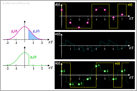
$\text{Example 1:}$ Let the total frequency response $H_{\rm K}(f) \cdot H_{\rm E}(f) = H_{\rm G}(f)$ be Gaussian with the cutoff frequency $f_{\rm G} = 0.3/T$. For NRZ rectangular pulses, this then yields the basic pulse $g_d(t)$ sketched in pink.
⇒ Shown on the left are the basic pulses $g_w(t)$ and $g_k(t)$ with ideal decision feedback, based on the detection time $T_{\rm D} = 0$ and the delay time $T_{\rm V} = T/2$.
⇒ The right pictures from [Söd01][1] – all without consideration of the noise – make clear that by the compensation of all pulse trailers by means of the correction signal $w(t)$, the distances of the useful signal samples $d_{\rm S}(\nu \cdot T)$ from the decision threshold $E = 0$ are changed.
- Particularly small distances, such as at times $t = 6T$ and $t = 7T$, are significantly increased and thus their error probabilities are greatly reduced (arrows pointing away from the threshold).
- In contrast, the samples further away from the threshold value $E = 0$ in the signal $d(t)$ are shifted towards the threshold and their falsification probabilities are thus slightly increased. This can be seen, for example, for time $t = 5T$.
Eye opening and error probability with DFE
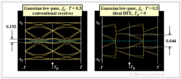
We now consider the eye diagrams
- without DFE (left graph) and
- with ideal DFE (right graph).
We assume the same conditions as in the last section, so that the following basic pulse values are present:
- $$g_0 = g_d(t=0) = 0.548 \cdot s_0,$$
- $$g_1 = g_d(t=T) = 0.214 \cdot s_0 = g_{-1} \hspace{0.05cm},$$
- $$g_2 = g_d(t=2\hspace{0.05cm}T) = 0.012 \cdot s_0 = g_{-2} \hspace{0.05cm},$$
- $$g_3 = g_{-3} = \text{...} \approx 0 \hspace{0.05cm}.$$
These two eye diagrams can be interpreted as follows:
- For the conventional receiver (without DFE), with binary bipolar redundancy-free coding considering symmetry:
- $${\ddot{o}(T_{\rm D} = 0 )} = {2} \cdot \big [ g_0 - | g_{-1}| - | g_{-2}| - | g_{1}| - | g_{2}|\big ] = {2} \cdot \big [ g_0 - 2 \cdot g_{1} - 2 \cdot g_{2}\big ]= 0.192 \cdot s_0 \hspace{0.05cm}.$$
- On the other hand, for ideal DFE, the two trailers $g_1$ and $g_2$ are fully compensated and we obtain for the vertical eye opening:
- $${\ddot{o}(T_{\rm D} = 0 )} = {2} \cdot \big [ g_0 - | g_{-1}| - |g_{-2}|\big ] = {2} \cdot \big [ g_0 - g_{1} - g_{2}\big ]= 0.644 \cdot s_0 \hspace{0.05cm}.$$
- Since the correction signal $w(t)$ is derived from the decision and thus noise-free signal $v(t)$, the noise rms value $\sigma_d$ is not changed by the decision feedback. Thus, the SNR gain due to the DFE is
- $$G_{\rm DFE}= 20 \cdot {\rm lg}\hspace{0.1cm}\frac{0.644}{0.192} \approx 10.5\,{\rm dB} \hspace{0.05cm}.$$
$\text{Conclusion:}$ For a coaxial cable with characteristic cable attenuation $a_\star = 80 \ \rm dB$ and $10 \cdot \lg \ (E_{\rm B}/N_0) = 80 \ \rm dB$,
this SNR gain means that the worst-case error probability $p_{\rm U}$ is reduced by DFE from $7\%$ to about $4 \cdot 10^{-7}$ – a quite remarkable improvement.
Optimization of a transmission system with DFE
The last section has already made clear that the DFE already causes an enormous SNR gain if
- a fixed cutoff frequency $f_{\rm G}$ and
- the fixed detection time $T_{\rm D} = 0$
is assumed. However, the system can be further improved if the two parameters $f_{\rm G}$ and $T_{\rm D}$ are optimized together.
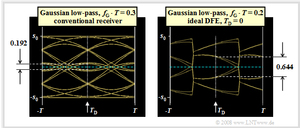
The graph shows the eye diagrams without noise for
- $f_{\rm G} \cdot T = 0.3$ (left),
- $f_{\rm G} \cdot T = 0.2$ (right).
For the diagram and the following calculations are still assumed:
- the characteristic cable attenuation $a_\star = 80 \ \rm dB$,
- the AWGN parameter $10 \cdot \lg \ (E_{\rm B}/N_0) = 80 \ \rm dB$
$($with $E_{\rm B} = s_0^2 \cdot T)$.
The left diagram is largely identical – except for the detection time $T_{\rm D}$ – to the right diagram in the last section. The optimization results can be summarized as follows:
- With $f_{\rm G} \cdot T = 0.3$, by shifting the detection time to $T_\text{D, opt} = -0.3T$, the eye opening can be increased to $\ddot{o}(T_\text{D, opt}) = 0.779 \cdot s_0 $.
- Compared to $T_{\rm D} = 0$ $($see last section$)$, this results in a further SNR gain of $G_{T_\text{D, opt}}= 20 \cdot {\rm lg}\hspace{0.1cm}{0.779}/{644} \approx 1.65\,{\rm dB} \hspace{0.05cm}.$
- The worst-case error probability is now found to be $p_{\rm U} \approx 1.3 \cdot 10^{-9}$ $($versus $4 \cdot 10^{-7})$.
With the DFE receiver, however, you can further reduce the cutoff frequency. The reason is the better noise behavior with a smaller cutoff frequency.
- For example, the normalized noise rms value results instead of $\sigma_d/s_0 = 0.065$ $($for $f_{\rm G} \cdot T = 0.3)$ to $\sigma_d/s_0 = 0.010$ $($for $f_{\rm G} \cdot T = 0.2)$.
- Thus, with $f_{\rm G} \cdot T = 0.2$ and $T_{\rm D} = 0$ the small but nonzero eye opening $\ddot{o}_{\rm norm} = 0.152$ is obtained, which together with the very favorable noise rms value leads to the worst-case SNR $10 \cdot \lg \ \rho_{\rm U} = 17.6 \ \rm dB$ ⇒ worst-case error probabilty $p_{\rm U} \approx 1.6 \cdot 10^{-14}$.
- By combining the cutoff frequency $f_{\rm G} \cdot T = 0.2$ with the detection time $T_{\rm D} = -T/2$, one finally obtains the optimal system configuration with the normalized eye opening $\ddot{o}_{\rm norm} = 0.368$ and the worst-case SNR $10 \cdot \lg \ \rho_{\rm U} = 25.3 \ \rm dB$.
- Thus (practically) $p_{\rm U}\approx 0$. However, this configuration is not relevant in practice: Already a minimal tolerance of the system parameters leads to a "closed eye".
Realization aspects of the decision feedback
As an essential result of the last chapter "Linear Nyquist Equalization" and the current chapter "Decision Feedback" the following approach is recommended:
$\text{Conclusion:}$ For a transmission system over copper lines $($coaxial cable, two-wire line$)$, the following system variants are particularly suitable due to the achievable signal–to–noise ratio at the decision:
- a multi-level system $($for example $M = 4)$ and the optimal Nyquist equalization to compensate for the strong intersymbol interference caused by the linear channel distortions;
- a binary system with relatively small bandwidth of the total frequency response $H_{\rm G}(f) = H_{\rm K}(f) \cdot H_{\rm E}(f)$ and a non-linear decision with DFE.
Both system variants provide comparably good results under idealized conditions. But it should be noted, that large degradations can occur due to realization inaccuracies in both systems, which are mentioned here using the DFE system as an example:
- Since no DC signal can be transmitted via the telephone network, but $H_{\rm K}(f=0) = 1$ is assumed for our calculations, a "DC signal recovery" is required at the receiver. This statement applies in the same way to the quaternary Nyquist system.
- In the DFE system, the compensation pulse $g_w(t)$ must exactly replicate the pre-equalized basic pulse $g_d(t)$. This is especially difficult when $g_d(t)$ is very broad $($small cutoff frequency, e.g. $f_{\rm G} \cdot T = 0.2)$ and the optimization yields the detection time $T_\text{D, opt} = -T/2$.
- If a wrong decision occurs due to a large noise value, the subsequent symbols will also be falsified with a high probability. However, there are always symbol sequences which interrupt this "propogation of uncertainty".
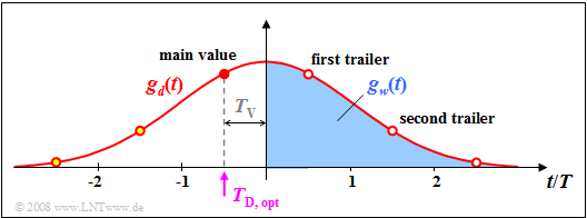
$\text{Example 2:}$ The graph shows the basic pulse $g_d(t)$
- for the cutoff frequency $f_{\rm G} \cdot T = 0.2$ (red curve) and
- the compensation pulse $g_w(t)$ for $T_\text{D} = -T/2$ (filled in blue).
Here, a delay time $T_\text{V} = -T/2$ between decision and start of signal correction is considered. It can be seen:
- For $T_\text{D} = -T/2$ the first trailer $g_d(T_\text{D} +T) = g_d(T/2)$ is exactly as large as the main value $g_d(T_\text{D}) = g_d(-T/2)$.
- If it is not possible to fully compensate all the trailers, this quickly results in a closed eye and thus, in the worst–case error probability $p_{\rm U} \approx 50\%$.
Decision feedback with delay filter
For a circuit realization it is sufficient if the basic corrected pulse $g_k(t)$ becomes zero only at the equidistant detection times $T_\text{D} +\nu \cdot T$.
One realization possibility is thus an asymmetric delay filter according to the adjacent diagram,
- whose order $N$ (number of filter coefficients), and
- whose filter coefficients $ k_\nu$ $($mit $\nu = 1$, ... , $N)$
are determined by the pulse $g_d(t)$ and the detection time $T_\text{D}$.
This DFE realization has the following properties:
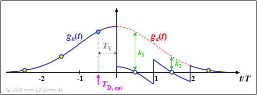
- Since the output signal $v(t)$ is rectangular, the compensation pulse $g_w(t)$ is staircase shaped.
- With proper dimensioning of the filter coefficients $k_\nu$,
for $\nu = 1$, ... , $N$:
- $$g_w(T_{\rm D} + \nu \cdot T) = g_d(T_{\rm D} + \nu \cdot T) \hspace{0.3cm}\Rightarrow\hspace{0.3cm} g_k(T_{\rm D} + \nu \cdot T) = 0 \hspace{0.05cm}.$$
- At detection time $T_\text{D}$, the vertical eye opening is exactly the same as for ideal DFE. A disadvantage is a smaller horizontal eye opening.
$\text{Example 3:}$ The graph shows the basic pulses $g_d(t)$ and $g_w(t)$ for decision feedback with a second order delay filter. The same conditions apply as for the example in the last section: $f_{\rm G} \cdot T = 0.2$ and $T_\text{D} = -T/2$. One can see:
- Because of the order $N = 2$, only the first two trailers $g_d(0.5T)$ and $g_d(1.5T)$ are compensated here.
- The third trailer $g_d(2.5T)$ could be compensate by a further filter coefficient $k_3$.
- In contrast, the precursors $g_d(-1.5T)$ and $g_d(-2.5T)$ cannot be compensated in principle.
Exercises for the chapter
Exercise 3.8: Delay Filter DFE Realization
Exercise 3.8Z: Optimal Detection Time for DFE
References
- ↑ Söder, G.: Simulation digitaler Übertragungssysteme. Anleitung zum gleichnamigen Praktikum. Lehrstuhl für Nachrichtentechnik, Technische Universität München, 2001.
