Difference between revisions of "Aufgaben:Exercise 5.2: Error Correlation Function"
| Line 2: | Line 2: | ||
{{quiz-Header|Buchseite=Digital_Signal_Transmission/Parameters_of_Digital_Channel_Models}} | {{quiz-Header|Buchseite=Digital_Signal_Transmission/Parameters_of_Digital_Channel_Models}} | ||
| − | [[File:P_ID1854__Dig_A_5_2_version1.png|right|frame| | + | [[File:P_ID1854__Dig_A_5_2_version1.png|right|frame|Error distance probability & error correlation function]] |
For the characterization of digital channel models one uses among other things | For the characterization of digital channel models one uses among other things | ||
| − | * the error correlation function (ECF) | + | * the "error correlation function" $\rm (ECF)$ |
:$$\varphi_{e}(k) = {\rm E}\big[e_{\nu} \cdot e_{\nu + | :$$\varphi_{e}(k) = {\rm E}\big[e_{\nu} \cdot e_{\nu + | ||
k}\big]\hspace{0.05cm}, \hspace{0.2cm} k \ge 0\hspace{0.05cm},$$ | k}\big]\hspace{0.05cm}, \hspace{0.2cm} k \ge 0\hspace{0.05cm},$$ | ||
| − | * the error distance probabilities | + | * the "error distance probabilities" |
:$${\rm Pr}( a =k) \hspace{0.05cm}, \hspace{0.2cm} k \ge | :$${\rm Pr}( a =k) \hspace{0.05cm}, \hspace{0.2cm} k \ge | ||
1\hspace{0.05cm}.$$ | 1\hspace{0.05cm}.$$ | ||
Here denote: | Here denote: | ||
| − | * $〈e_{\rm \nu}〉$ is the error sequence with $e_{\rm \nu} ∈ \{0, 1\}$. | + | * $〈e_{\rm \nu}〉$ is the error sequence with $e_{\rm \nu} ∈ \{0, 1\}$. |
| − | * $a$ indicates the error distance. | + | |
| + | * $a$ indicates the error distance with $a_{\rm \nu} ∈ \{0, 1, 2, \text{...} \}$. | ||
| − | Two directly consecutive | + | Two directly consecutive symbol errors are thus characterized by the error distance $a = 1$. |
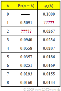
The table shows exemplary values of the error distance probabilities ${\rm Pr}(a = k)$ as well as the error correlation function $\varphi_e(k)$. | The table shows exemplary values of the error distance probabilities ${\rm Pr}(a = k)$ as well as the error correlation function $\varphi_e(k)$. | ||
| Line 26: | Line 27: | ||
| − | + | Note: The exercise covers the subject matter of the chapter [[Digital_Signal_Transmission/Parameters_of_Digital_Channel_Models|"Parameters of Digital Channel Models"]]. | |
| − | |||
| − | |||
| − | |||
| Line 35: | Line 33: | ||
===Questions=== | ===Questions=== | ||
<quiz display=simple> | <quiz display=simple> | ||
| − | {Which value results for the | + | {Which value results for the mean error probability? |
|type="{}"} | |type="{}"} | ||
$p_{\rm M} \ = \ ${ 0.1 3% } | $p_{\rm M} \ = \ ${ 0.1 3% } | ||
| Line 43: | Line 41: | ||
${\rm E}\big[a\big] \ = \ ${ 10 3% } | ${\rm E}\big[a\big] \ = \ ${ 10 3% } | ||
| − | {Calculate the value of the error correlation function (ECF) for $k = 1$. | + | {Calculate the value of the error correlation function \rm (ECF)$ for $k = 1$. |
|type="{}"} | |type="{}"} | ||
$\varphi_e(k = 1) \ = \ ${ 0.0309 3% } | $\varphi_e(k = 1) \ = \ ${ 0.0309 3% } | ||
Revision as of 17:32, 3 September 2022
For the characterization of digital channel models one uses among other things
- the "error correlation function" $\rm (ECF)$
- $$\varphi_{e}(k) = {\rm E}\big[e_{\nu} \cdot e_{\nu + k}\big]\hspace{0.05cm}, \hspace{0.2cm} k \ge 0\hspace{0.05cm},$$
- the "error distance probabilities"
- $${\rm Pr}( a =k) \hspace{0.05cm}, \hspace{0.2cm} k \ge 1\hspace{0.05cm}.$$
Here denote:
- $〈e_{\rm \nu}〉$ is the error sequence with $e_{\rm \nu} ∈ \{0, 1\}$.
- $a$ indicates the error distance with $a_{\rm \nu} ∈ \{0, 1, 2, \text{...} \}$.
Two directly consecutive symbol errors are thus characterized by the error distance $a = 1$.
The table shows exemplary values of the error distance probabilities ${\rm Pr}(a = k)$ as well as the error correlation function $\varphi_e(k)$.
- Some data are missing in the table.
- These values are to be calculated from the given values.
Note: The exercise covers the subject matter of the chapter "Parameters of Digital Channel Models".
Questions
Solution
- $$\varphi_{e}(k = 0) = {\rm E}[e_{\nu}^2 ]= {\rm E}[e_{\nu} ]= p_{\rm M} \hspace{0.3cm} \Rightarrow \hspace{0.3cm}p_{\rm M}\hspace{0.15cm}\underline { = 0.1} \hspace{0.05cm}.$$
(2) The mean error distance is equal to the reciprocal of the mean error probability. That is:
- $${\rm E}\big[a\big] = 1/p_{\rm M} \ \underline {= 10}.$$
(3) According to the definition equation and "Bayes' theorem", the following result is obtained:
- $$\varphi_{e}(k = 1) \hspace{-0.1cm} \ = \ \hspace{-0.1cm} {\rm E}[e_{\nu} \cdot e_{\nu + 1}] = {\rm E}[(e_{\nu} = 1) \cdot (e_{\nu + 1}=1)]={\rm Pr}(e_{\nu + 1}=1 \hspace{0.05cm}|\hspace{0.05cm} e_{\nu} = 1) \cdot {\rm Pr}(e_{\nu} = 1) \hspace{0.05cm}.$$
- The first probability is equal to ${\rm Pr}(a = 1)$ and the second probability is equal to $p_{\rm M}$:
- $$\varphi_{e}(k = 1) = 0.3091 \cdot 0.1\hspace{0.15cm}\underline { = 0.0309} \hspace{0.05cm}.$$
(4) The ECF value $\varphi_e(k = 2)$ can be interpreted (approximately) as follows:
- $$\varphi_{e}(k = 2) ={\rm Pr}(e_{\nu + 2}=1 \hspace{0.05cm}|\hspace{0.05cm} e_{\nu} = 1) \cdot p_{\rm M} \hspace{0.3cm} \Rightarrow \hspace{0.3cm}{\rm Pr}(e_{\nu + 2}=1 \hspace{0.05cm}|\hspace{0.05cm} e_{\nu} = 1) = \frac{\varphi_{e}(k = 2)}{p_{\rm M}} = \frac{0.0267}{0.1} = 0.267\hspace{0.05cm}.$$
This probability is composed of "At time $\nu+1$ an error occurs" and "At time $\nu+1$ there is no error":
- $${\rm Pr}(e_{\nu + 2}=1 \hspace{0.05cm}|\hspace{0.05cm} e_{\nu} = 1) = {\rm Pr}( a =1) \cdot {\rm Pr}( a =1) + {\rm Pr}( a =2)\hspace{0.3cm} \Rightarrow \hspace{0.3cm}{\rm Pr}( a =2)= 0.267 - 0.3091^2 \hspace{0.15cm}\underline {= 0.1715}\hspace{0.05cm}.$$
In the calculation, it was assumed that the individual error distances are statistically independent of each other.
- However, this assumption is valid only for a special class of channel models called "renewing".
- The burst error model considered here does not satisfy this condition.
- The actual probability ${\rm Pr}(a = 2) = 0.1675$ therefore deviates slightly from the value calculated here $(0.1715)$.
