Difference between revisions of "Aufgaben:Exercise 4.4: Conventional Entropy and Differential Entropy"
m (Text replacement - "„" to """) |
|||
| (13 intermediate revisions by 3 users not shown) | |||
| Line 1: | Line 1: | ||
| − | {{quiz-Header|Buchseite= | + | {{quiz-Header|Buchseite=Information_Theory/Differential_Entropy |
}} | }} | ||
| − | [[File:P_ID2878__Inf_A_4_4.png|right|frame| | + | [[File:P_ID2878__Inf_A_4_4.png|right|frame|Two uniform distributions]] |
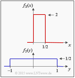
| − | + | We consider the two continuous random variables $X$ and $Y$ with probability density functions $f_X(x)$ and $f_Y(y)$. For these random variables one can | |
| − | * | + | * not specify the conventional entropies $H(X)$ and $H(Y)$ , respectively, |
| − | * | + | * but the differential entropies $h(X)$ and $h(Y)$. |
| − | + | We also consider two discrete random variables: | |
| − | * | + | *The variable $Z_{X,\hspace{0.05cm}M}$ is obtained by (suitably) quantizing the random quantity $X$ with the quantization level number $M$ <br>⇒ quantization interval width ${\it \Delta} = 0.5/M$. |
| − | * | + | * The variable $Z_{Y,\hspace{0.05cm}M}$ is obtained after quantization of the random quantity $Y$ with the quantization level number $M$ <br>⇒ quantization interval width ${\it \Delta} = 2/M$. |
| − | + | The probability density functions $\rm (PDF)$ of these discrete random variables are each composed of $M$ Dirac functions whose momentum weights are given by the interval areas of the associated continuous random variables. | |
| − | + | From this, the entropies $H(Z_{X,\hspace{0.05cm}M})$ and $H(Z_{Y,\hspace{0.05cm}M})$ can be determined in the conventional way according to the section [[Information_Theory/Einige_Vorbemerkungen_zu_zweidimensionalen_Zufallsgrößen#Probability_mass_function_and_entropy|Probability mass function and entropy]] . | |
| − | + | In the section [[Information_Theory/Differentielle_Entropie#Entropy_of_continuous_random_variables_after_quantization|Entropy of value-ontinuous random variables after quantization]], an approximation was also given. For example: | |
:$$H(Z_{X, \hspace{0.05cm}M}) \approx -{\rm log}_2 \hspace{0.1cm} ({\it \Delta}) + h(X)\hspace{0.05cm}. $$ | :$$H(Z_{X, \hspace{0.05cm}M}) \approx -{\rm log}_2 \hspace{0.1cm} ({\it \Delta}) + h(X)\hspace{0.05cm}. $$ | ||
| − | * | + | *In the course of the task it will be shown that in the case of rectangular PDF ⇒ uniform distribution this "approximation" gives the same result as the direct calculation. |
| − | * | + | *But in the general case – so in [[Information_Theory/Differentielle_Entropie#Entropy_of_continuous_random_variables_after_quantization|$\text{Example 2}$]] with triangular PDF – this equation is in fact only an approximation, which agrees with the actual entropy $H(Z_{X,\hspace{0.05cm}M})$ only in the limiting case ${\it \Delta} \to 0$ . |
| Line 31: | Line 31: | ||
| − | + | Hints: | |
| − | + | *The exercise belongs to the chapter [[Information_Theory/Differentielle_Entropie|Differential Entropy]]. | |
| − | * | + | *Useful hints for solving this task can be found in particular in the section [[Information_Theory/Differentielle_Entropie#Entropy_of_continuous_random_variables_after_quantization|Entropy of continuous random variables after quantization]]. |
| − | * | ||
| − | === | + | ===Questions=== |
<quiz display=simple> | <quiz display=simple> | ||
| − | { | + | {Calculate the differential entropy $h(X)$. |
|type="{}"} | |type="{}"} | ||
$ h(X) \ = \ $ { -1.03--0.97 } $\ \rm bit$ | $ h(X) \ = \ $ { -1.03--0.97 } $\ \rm bit$ | ||
| − | { | + | {Calculate the differential entropy $h(Y)$. |
|type="{}"} | |type="{}"} | ||
$ h(Y) \ = \ $ { 1 3% } $\ \rm bit$ | $ h(Y) \ = \ $ { 1 3% } $\ \rm bit$ | ||
| − | { | + | {Calculate the entropy of the discrete random variables $Z_{X,\hspace{0.05cm}M=4}$ using the direct method</u>. |
|type="{}"} | |type="{}"} | ||
$H(Z_{X,\hspace{0.05cm}M=4})\ = \ $ { 2 3% } $\ \rm bit$ | $H(Z_{X,\hspace{0.05cm}M=4})\ = \ $ { 2 3% } $\ \rm bit$ | ||
| − | { | + | {Calculate the entropy of the discrete random variables $Z_{X,\hspace{0.05cm}M=4}$ using the given approximation</u>. |
|type="{}"} | |type="{}"} | ||
$H(Z_{X,\hspace{0.05cm}M=4})\ = \ $ { 2 3% } $\ \rm bit$ | $H(Z_{X,\hspace{0.05cm}M=4})\ = \ $ { 2 3% } $\ \rm bit$ | ||
| − | { | + | {Calculate the entropy of the discrete random variable $Z_{Y,\hspace{0.05cm}M=8}$ with the given approximation</u>. |
|type="{}"} | |type="{}"} | ||
$H(Z_{Y,\hspace{0.05cm}M=8})\ = \ $ { 3 3% } $\ \rm bit$ | $H(Z_{Y,\hspace{0.05cm}M=8})\ = \ $ { 3 3% } $\ \rm bit$ | ||
| − | { | + | {Which of the following statements are true? |
|type="[]"} | |type="[]"} | ||
| − | + | + | + The entropy of a discrete value random variable $Z$ is always $H(Z) \ge 0$. |
| − | - | + | - The differential entropy of a continuous value random variable $X$ is always $h(X) \ge 0$. |
| Line 71: | Line 70: | ||
</quiz> | </quiz> | ||
| − | === | + | ===Solution=== |
{{ML-Kopf}} | {{ML-Kopf}} | ||
| − | '''(1)''' | + | '''(1)''' According to the corresponding theory section, with $x_{\rm min} = 0$ and $x_{\rm max} = 1/2$: |
:$$h(X) = {\rm log}_2 \hspace{0.1cm} (x_{\rm max} - x_{\rm min}) = {\rm log}_2 \hspace{0.1cm} (1/2) \hspace{0.15cm}\underline{= - 1\,{\rm bit}}\hspace{0.05cm}.$$ | :$$h(X) = {\rm log}_2 \hspace{0.1cm} (x_{\rm max} - x_{\rm min}) = {\rm log}_2 \hspace{0.1cm} (1/2) \hspace{0.15cm}\underline{= - 1\,{\rm bit}}\hspace{0.05cm}.$$ | ||
| − | '''(2)''' | + | '''(2)''' On the other hand, with $y_{\rm min} = -1$ and $y_{\rm max} = +1$ the differential entropy of the random variable $Y$ is given by: |
:$$h(Y) = {\rm log}_2 \hspace{0.1cm} (y_{\rm max} - y_{\rm min}) = {\rm log}_2 \hspace{0.1cm} (2) \hspace{0.15cm}\underline{= + 1\,{\rm bit}}\hspace{0.05cm}. $$ | :$$h(Y) = {\rm log}_2 \hspace{0.1cm} (y_{\rm max} - y_{\rm min}) = {\rm log}_2 \hspace{0.1cm} (2) \hspace{0.15cm}\underline{= + 1\,{\rm bit}}\hspace{0.05cm}. $$ | ||
| − | [[File:P_ID2879__Inf_A_4_4c.png|right|frame| | + | [[File:P_ID2879__Inf_A_4_4c.png|right|frame|Quantized random variable $Z_{X, \ M = 4}$]] |
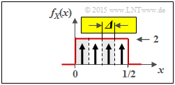
| − | '''(3)''' | + | '''(3)''' The adjacent graph illustrates the best possible quantization of random variable $X$ with quantization level number $M = 4$ ⇒ random variable $Z_{X, \ M = 4}$: |
| − | * | + | *The interval width here is equal to ${\it \Delta} = 0.5/4 = 1/8$. |
| − | * | + | *The possible values (at the center of the interval, respectively) are $z \in \{0.0625,\ 0.1875,\ 0.3125,\ 0.4375\}$. |
| − | + | Using the probability mass function, the <u>direct entropy calculation</u> gives $P_Z(Z) = \big [1/4,\ \text{...} , \ 1/4 \big]$: | |
:$$H(Z_{X, \ M = 4}) = {\rm log}_2 \hspace{0.1cm} (4) \hspace{0.15cm}\underline{= 2\,{\rm bit}} | :$$H(Z_{X, \ M = 4}) = {\rm log}_2 \hspace{0.1cm} (4) \hspace{0.15cm}\underline{= 2\,{\rm bit}} | ||
\hspace{0.05cm}.$$ | \hspace{0.05cm}.$$ | ||
| − | + | With the <u>approximation</u>, considering the result of '''(1)''', we obtain: | |
:$$H(Z_{X,\hspace{0.05cm} M = 4}) \approx -{\rm log}_2 \hspace{0.1cm} ({\it \Delta}) + h(X) = | :$$H(Z_{X,\hspace{0.05cm} M = 4}) \approx -{\rm log}_2 \hspace{0.1cm} ({\it \Delta}) + h(X) = | ||
3\,{\rm bit} +(- 1\,{\rm bit})\hspace{0.15cm}\underline{= 2\,{\rm bit}}\hspace{0.05cm}. $$ | 3\,{\rm bit} +(- 1\,{\rm bit})\hspace{0.15cm}\underline{= 2\,{\rm bit}}\hspace{0.05cm}. $$ | ||
| − | <i> | + | <i>Note:</i> Only in the case of uniform distribution, the approximation gives exactly the same result as the direct calculation, i.e. the actual entropy. |
| − | [[File:P_ID2880__Inf_A_4_4d.png|right|frame| | + | [[File:P_ID2880__Inf_A_4_4d.png|right|frame|Quantized random variable $Z_{Y, \ M = 4}$]] |
<br> | <br> | ||
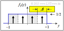
| − | '''(4)''' | + | '''(4)''' From the second graph, one can see the similarities / differences to subtask '''(3)''': |
| − | * | + | * The quantization parameter is now ${\it \Delta} = 2/4 = 1/2$. |
| − | * | + | * The possible values are now $z \in \{\pm 0.75,\ \pm 0.25\}$. |
| − | * | + | * Thus, here the "approximation" (as well as the direct calculation) gives the result: |
:$$H(Z_{Y,\hspace{0.05cm} M = 4}) \approx -{\rm log}_2 \hspace{0.1cm} ({\it \Delta}) + h(Y) = | :$$H(Z_{Y,\hspace{0.05cm} M = 4}) \approx -{\rm log}_2 \hspace{0.1cm} ({\it \Delta}) + h(Y) = | ||
1\,{\rm bit} + 1\,{\rm bit}\hspace{0.15cm}\underline{= 2\,{\rm bit}}\hspace{0.05cm}.$$ | 1\,{\rm bit} + 1\,{\rm bit}\hspace{0.15cm}\underline{= 2\,{\rm bit}}\hspace{0.05cm}.$$ | ||
| − | [[File:P_ID2881__Inf_A_4_4e.png|right|frame| | + | [[File:P_ID2881__Inf_A_4_4e.png|right|frame|Quantized random variable $Z_{Y, \ M = 8}$]] |
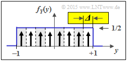
| − | '''(5)''' | + | '''(5)''' In contrast to subtask '''(5)''': ${\it \Delta} = 1/4$ is now valid. From this follows for the "approximation": |
:$$H(Z_{Y,\hspace{0.05cm} M = 8}) \approx -{\rm log}_2 \hspace{0.1cm} ({\it \Delta}) + h(Y) = | :$$H(Z_{Y,\hspace{0.05cm} M = 8}) \approx -{\rm log}_2 \hspace{0.1cm} ({\it \Delta}) + h(Y) = | ||
2\,{\rm bit} + 1\,{\rm bit}\hspace{0.15cm}\underline{= 3\,{\rm bit}}\hspace{0.05cm}.$$ | 2\,{\rm bit} + 1\,{\rm bit}\hspace{0.15cm}\underline{= 3\,{\rm bit}}\hspace{0.05cm}.$$ | ||
| − | + | Again, one gets the same result as in the direct calculation. | |
| − | + | ||
| − | '''(6)''' | + | |
| − | * | + | '''(6)''' Only <u>statement 1</u> is correct: |
| − | * | + | * The entropy $H(Z)$ of a discrete random variable $Z = \{z_1, \ \text{...} \ , z_M\}$ is never negative. |
| + | *For example, the limiting case $H(Z) = 0$ results for ${\rm Pr}(Z = z_1) = 1$ and ${\rm Pr}(Z = z_\mu) = 0$ for $2 \le \mu \le M$. | ||
| − | * | + | * In contrast, the differential entropy $h(X)$ of a continuous value random variable $X$ can be as follows: |
| − | ** $h(X) < 0$ $($ | + | ** $h(X) < 0$ $($subtask 1$)$, |
| − | ** $h(X) > 0$ $($ | + | ** $h(X) > 0$ $($subtask 2$)$, or even |
| − | **$h(X) = 0$ $($ | + | **$h(X) = 0$ $($for example fo $x_{\rm min} = 0$ and $x_{\rm max} = 1)$. |
{{ML-Fuß}} | {{ML-Fuß}} | ||
| Line 127: | Line 127: | ||
| − | [[Category:Information Theory: Exercises|^4.1 | + | [[Category:Information Theory: Exercises|^4.1 Differential Entropy^]] |
Latest revision as of 14:44, 17 November 2022
We consider the two continuous random variables $X$ and $Y$ with probability density functions $f_X(x)$ and $f_Y(y)$. For these random variables one can
- not specify the conventional entropies $H(X)$ and $H(Y)$ , respectively,
- but the differential entropies $h(X)$ and $h(Y)$.
We also consider two discrete random variables:
- The variable $Z_{X,\hspace{0.05cm}M}$ is obtained by (suitably) quantizing the random quantity $X$ with the quantization level number $M$
⇒ quantization interval width ${\it \Delta} = 0.5/M$. - The variable $Z_{Y,\hspace{0.05cm}M}$ is obtained after quantization of the random quantity $Y$ with the quantization level number $M$
⇒ quantization interval width ${\it \Delta} = 2/M$.
The probability density functions $\rm (PDF)$ of these discrete random variables are each composed of $M$ Dirac functions whose momentum weights are given by the interval areas of the associated continuous random variables.
From this, the entropies $H(Z_{X,\hspace{0.05cm}M})$ and $H(Z_{Y,\hspace{0.05cm}M})$ can be determined in the conventional way according to the section Probability mass function and entropy .
In the section Entropy of value-ontinuous random variables after quantization, an approximation was also given. For example:
- $$H(Z_{X, \hspace{0.05cm}M}) \approx -{\rm log}_2 \hspace{0.1cm} ({\it \Delta}) + h(X)\hspace{0.05cm}. $$
- In the course of the task it will be shown that in the case of rectangular PDF ⇒ uniform distribution this "approximation" gives the same result as the direct calculation.
- But in the general case – so in $\text{Example 2}$ with triangular PDF – this equation is in fact only an approximation, which agrees with the actual entropy $H(Z_{X,\hspace{0.05cm}M})$ only in the limiting case ${\it \Delta} \to 0$ .
Hints:
- The exercise belongs to the chapter Differential Entropy.
- Useful hints for solving this task can be found in particular in the section Entropy of continuous random variables after quantization.
Questions
Solution
- $$h(X) = {\rm log}_2 \hspace{0.1cm} (x_{\rm max} - x_{\rm min}) = {\rm log}_2 \hspace{0.1cm} (1/2) \hspace{0.15cm}\underline{= - 1\,{\rm bit}}\hspace{0.05cm}.$$
(2) On the other hand, with $y_{\rm min} = -1$ and $y_{\rm max} = +1$ the differential entropy of the random variable $Y$ is given by:
- $$h(Y) = {\rm log}_2 \hspace{0.1cm} (y_{\rm max} - y_{\rm min}) = {\rm log}_2 \hspace{0.1cm} (2) \hspace{0.15cm}\underline{= + 1\,{\rm bit}}\hspace{0.05cm}. $$
(3) The adjacent graph illustrates the best possible quantization of random variable $X$ with quantization level number $M = 4$ ⇒ random variable $Z_{X, \ M = 4}$:
- The interval width here is equal to ${\it \Delta} = 0.5/4 = 1/8$.
- The possible values (at the center of the interval, respectively) are $z \in \{0.0625,\ 0.1875,\ 0.3125,\ 0.4375\}$.
Using the probability mass function, the direct entropy calculation gives $P_Z(Z) = \big [1/4,\ \text{...} , \ 1/4 \big]$:
- $$H(Z_{X, \ M = 4}) = {\rm log}_2 \hspace{0.1cm} (4) \hspace{0.15cm}\underline{= 2\,{\rm bit}} \hspace{0.05cm}.$$
With the approximation, considering the result of (1), we obtain:
- $$H(Z_{X,\hspace{0.05cm} M = 4}) \approx -{\rm log}_2 \hspace{0.1cm} ({\it \Delta}) + h(X) = 3\,{\rm bit} +(- 1\,{\rm bit})\hspace{0.15cm}\underline{= 2\,{\rm bit}}\hspace{0.05cm}. $$
Note: Only in the case of uniform distribution, the approximation gives exactly the same result as the direct calculation, i.e. the actual entropy.
(4) From the second graph, one can see the similarities / differences to subtask (3):
- The quantization parameter is now ${\it \Delta} = 2/4 = 1/2$.
- The possible values are now $z \in \{\pm 0.75,\ \pm 0.25\}$.
- Thus, here the "approximation" (as well as the direct calculation) gives the result:
- $$H(Z_{Y,\hspace{0.05cm} M = 4}) \approx -{\rm log}_2 \hspace{0.1cm} ({\it \Delta}) + h(Y) = 1\,{\rm bit} + 1\,{\rm bit}\hspace{0.15cm}\underline{= 2\,{\rm bit}}\hspace{0.05cm}.$$
(5) In contrast to subtask (5): ${\it \Delta} = 1/4$ is now valid. From this follows for the "approximation":
- $$H(Z_{Y,\hspace{0.05cm} M = 8}) \approx -{\rm log}_2 \hspace{0.1cm} ({\it \Delta}) + h(Y) = 2\,{\rm bit} + 1\,{\rm bit}\hspace{0.15cm}\underline{= 3\,{\rm bit}}\hspace{0.05cm}.$$
Again, one gets the same result as in the direct calculation.
(6) Only statement 1 is correct:
- The entropy $H(Z)$ of a discrete random variable $Z = \{z_1, \ \text{...} \ , z_M\}$ is never negative.
- For example, the limiting case $H(Z) = 0$ results for ${\rm Pr}(Z = z_1) = 1$ and ${\rm Pr}(Z = z_\mu) = 0$ for $2 \le \mu \le M$.
- In contrast, the differential entropy $h(X)$ of a continuous value random variable $X$ can be as follows:
- $h(X) < 0$ $($subtask 1$)$,
- $h(X) > 0$ $($subtask 2$)$, or even
- $h(X) = 0$ $($for example fo $x_{\rm min} = 0$ and $x_{\rm max} = 1)$.


