Theory of Stochastic Signals/Cumulative Distribution Function

1. Theory of Stochastic Signals
2. Continuous Random Variables
3. Cumulative Distribution Function

• Previous page
• Next page

• Previous page
• Next page

Relationship between PDF and CDF

To describe random variables,  in addition to the  $\text{probability density function}$  $\rm (PDF)$,  we also use the  cumulative distribution function  $\rm (CDF)$  which is defined as follows:

$\text{Definition:}$  The  »cumulative distribution function«  $F_{x}(r)$  corresponds to the probability that the random variable  $x$  is less than or equal to a real number  $r$:

$$F_{x}(r) = {\rm Pr}( x \le r).$$

For a continuous random variable,  the following statements are possible regarding the CDF:

• The CDF is computable from the probability density function  $f_{x}(x)$  by integration.  It holds:

$$F_{x}(r) = \int_{-\infty}^{r}f_x(x)\,{\rm d}x.$$

• Since the PDF is never negative,  $F_{x}(r)$  increases at least weakly monotonically,  and always lies between the following limits:

$$F_{x}(r → \hspace{0.05cm} - \hspace{0.05cm} ∞) = 0, \hspace{0.5cm}F_{x}(r → +∞) = 1.$$

• Inversely,  the probability density function can be determined from the CDF by differentiation:

$$f_{x}(x)=\frac{{\rm d} F_{x}(r)}{{\rm d} r}\Bigg |_{\hspace{0.1cm}r=x}.$$

The addition  "$r = x$"  makes it clear that in our nomenclature the PDF argument is the random variable itself, while the CDF argument specifies any real variable  $r$ .

$\text{Notes on nomenclature:}$ 

If in the definitions of  $\rm PDF$  and  $\rm CDF$  we had distinguished

• between the random variable  $X$ 
• and the realizations  $x ∈ X$    ⇒   $f_{X}(x), F_{X}(x)$,

we would have the following nomenclature:

$$F_{X}(x) = {\rm Pr}(X \le x) = \int_{-\infty}^{x}f_{x}(\xi)\,{\rm d}\xi.$$

Unfortunately,  at the beginning of our  $\rm LNTwww$ project  (2001)  we decided to use our nomenclature for quite legitimate reasons,  which now  (2017)  cannot be changed,  also with regard to the realized learning videos.

So we stick with  $f_{x}(x)$  instead of  $f_{X}(x)$  as well as  $F_{x}(r)$  instead of  $F_{X}(x).$

CDF for continuous-valued random variables

The equations given in the last section apply only to continuous-valued random variables and will be illustrated here by an example.  In the next section it will be shown that for  $\text{discrete-valued random variables}$  the equations must be modified somewhat.

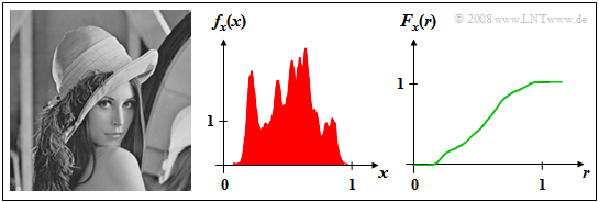
$\text{Example 1:}$  The left image shows the photo  "Lena",  which is often used as a test template for image coding procedures.

PDF and CDF of a continuous-valued image

• If this image is divided into  $256 × 256$  (image) pixels,  and the brightness is determined for each pixel,  a sequence  $〈x_ν〉$  of gray values is obtained whose length  $N = 256^2 = 65536$.
• The gray value  $x$  is a continuous-valued random variable,  where the assignment to numerical values is arbitrary.  For example,  let  "black"  be characterized by the value  $x = 0$  and  "white"  by  $x = 1$:  The value  $x =0.5$  then characterizes a medium gray coloration.

The middle diagram shows the PDF  $f_{x}(x)$  which is also often referred to in the literature as  "gray value statistics".

• It can be seen that in the original image some gray values are preferred and the two extreme values  $x =0$  ("deep black")  or  $x =1$  ("pure white")  occur very rarely.
• The distribution function  $F_{x}(r)$  of this continuous random variable is continuous and increases monotonically from  $0$  to  $1$  as the right figure shows. 
• For  $r \approx 0$  and  $r \approx 1$  the CDF is horizontal due to the lack of PDF components.

Note:   Strictly speaking,  for an image that can be displayed on a computer:  In contrast to an "analog" photograph:

1.   The gray value is always a discrete value random variable. 
2.   However,  with large resolution of the color information  ("color depth"),  this random variable can be approximated to be continuous in value.

The topic of this chapter is illustrated with examples in the  (German language)  learning video 
     "Zusammenhang zwischen WDF und VTF"  $\Rightarrow$ "Relationship between PDF and CDF".

CDF for discrete-valued random variables

For the CDF calculation of a discrete valued random variable  $x$  from its PDF,  a more general equation must always be assumed  Here, with the auxiliary variable  $\varepsilon > 0$:

$$F_{x}(r)=\lim_{\varepsilon\hspace{0.05cm}\to \hspace{0.05cm}0}\int_{-\infty}^{r+\varepsilon}f_x(x)\,{\rm d}x.$$

• The CDF calculation is here required by boundary value formation due to the  "less than/equal"  sign in the  $\text{general definition}$.
• If we also take into account that,  for a discrete valued random variable,  the PDF consists of a sum of weighted  $\text{Dirac delta functions}$,  we obtain:

$$F_{x}(r)=\lim_{\varepsilon\hspace{0.05cm}\to \hspace{0.05cm} 0}\int_{-\infty}^{r+\varepsilon}\sum\limits_{\mu= 1}^{ M}p_\mu\cdot \delta(x-x_\mu)\,{\rm d}x.$$

• If we interchange integration and summation in this equation,  and consider that integration over the Dirac delta function yields the step function,  we obtain:

$$F_{x}(r)=\sum\limits_{\mu= \rm 1}^{\it M}p_\mu\cdot \gamma_0 (r-x_\mu),\hspace{0.4cm}{\rm with} \hspace{0.4cm}\gamma_0(x)=\lim_{\epsilon\hspace{0.05cm}\to \hspace{0.05cm} 0}\int_{-\infty}^{x+\varepsilon}\delta (u)\,{\rm d} u = \left\{ \begin{array}{*{2}{c}} 0 \hspace{0.4cm} {\rm if}\hspace{0.1cm} x< 0,\\ 1 \hspace{0.4cm} {\rm if}\hspace{0.1cm}x\ge 0. \\ \end{array} \right.$$

It should be noted that:

• The function  $γ_0(x)$  differs from the  $\text{unit step function}$  $γ(x)$  often used in systems theory in that at the jump point  $x = 0$  the right-hand side limit  "one"  is valid  $($instead of the mean value  "$0.5$"  between left– and right–hand side limits$)$.
• With the above CDF definition,  the probability equation holds for continuous and discrete random variables equally,  and of course also for  "mixed random variables"  with discrete and continuous parts:

$${\rm Pr}(x_{\rm u}<x \le x_{\rm o})=F_x(x_{\rm o})-F_x(x_{\rm u}).$$

• For purely continuous random variables,  the  "less than"  sign and the  "less than/equal to"  sign could be substituted for each other here.

$${\rm Pr}(x_{\rm u}<x \le x_{\rm o}) ={\rm Pr}(x_{\rm u}\le x \le x_{\rm o}) ={\rm Pr}(x_{\rm u}\le x < x_{\rm o}) ={\rm Pr}(x_{\rm u}<x < x_{\rm o}).$$

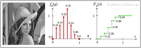
$\text{Example 2:}$  If the gray value of the  $\text{original Lena photo}$  is quantized by eight levels,  so that each pixel can be represented by three bits and transmitted digitally,  the discrete random variable  $q$  is obtained.   However, due to the quantization,  a part of the image information is lost,  which is reflected in the quantized image by clearly recognizable  "contours".

PDF and CDF of a discrete valued image

• The associated PDF  $f_{q}(q)$  is composed of  $M = 8$  Dirac delta functions, where,  in the quantization chosen here,  the possible gray levels are assigned the values  $q_\mu = (\mu - 1)/7$  with  $\mu = 1, 2,$ ... , $8$.
• The weights of the Dirac delta functions can be calculated from the PDF  $f_{x}(x)$  of the original image.  One obtains

$$p_\mu={\rm Pr}(q = q_\mu ) = {\rm Pr}(\frac{2\mu-\rm 3}{14}< {x} \le\frac{2\it \mu- \rm 1}{14}) $$

$$\Rightarrow \hspace{0.3cm} p_\mu={\rm Pr}(q = q_\mu ) = \int_{(2\it \mu- \rm 3)/14}^{(2\mu-1)/14}\it f_{x}{\rm (}x{\rm )}\,{\rm d}x.$$

• For the undefined areas  $(x<0$,   $x>1)$  is to be set  $f_{x}(x) = 0$ .
• Since in the original image the gray levels  $x ≈0$  ("very deep black")  or  $x ≈1$  ("almost pure white")  are largely missing,  $p_1 ≈ p_8 ≈ 0$ result.
• Thus,  only six Dirac delta functions are visible in the PDF.  The two missing Diracs at  $q = 0$  and  $q =1$  are only indicated by dots.
• The step-shaped CDF  $F_{q}(r)$  sketched on the right thus has six points of discontinuity,  where in each case the right-hand side limit is valid.

.

The topic of this chapter is illustrated with examples in the  (German language)  learning video 
     "Zusammenhang zwischen WDF und VTF"  $\Rightarrow$ "Relationship between PDF and CDF".

Exercises for the chapter

Exercise 3.2: CDF for Exercise_3.1

Exercise 3.2Z: Relationship between PDF and CDF