Difference between revisions of "Theory of Stochastic Signals/Two-Dimensional Gaussian Random Variables"
| (33 intermediate revisions by 6 users not shown) | |||
| Line 1: | Line 1: | ||
{{Header | {{Header | ||
| − | |Untermenü= | + | |Untermenü=Random Variables with Statistical Dependence |
| − | |Vorherige Seite= | + | |Vorherige Seite=Two-Dimensional Random Variables |
| − | |Nächste Seite= | + | |Nächste Seite=Linear Combinations of Random Variables |
}} | }} | ||
| − | == | + | ==Probability density function and cumulative distribution function== |
<br> | <br> | ||
| − | + | All previous statements of the fourth main chapter "Random Variables with Statistical Dependence" apply in general. | |
| − | * | + | |
| − | :$$f_{xy}(x,y)=\frac{\rm 1}{\rm 2\it\pi \cdot \sigma_x \cdot \sigma_y \sqrt{\rm 1-\rho_{\it xy}^2}}\cdot\exp\Bigg[-\frac{\rm 1}{\rm 2 (1-\it\rho_{xy}^{\rm 2} {\rm)}}\cdot(\frac {\it x^{\rm 2}}{\sigma_x^{\rm 2}}+\frac {\it y^{\rm 2}}{\sigma_y^{\rm 2}}-\rm 2\it\rho_{xy}\cdot\frac{x \cdot y}{\sigma_x \cdot \sigma_y}\rm ) \rm \Bigg].$$ | + | For the special case »'''Gaussian random variables'''« – the name goes back to the scientist [https://en.wikipedia.org/wiki/Carl_Friedrich_Gauss $\text{Carl Friedrich Gauss}$] – we can further note: |
| − | * | + | *The joint probability density function of a two-dimensional Gaussian random variable $(x, y)$ with mean values $m_x = 0$, $m_y = 0$ and correlation coefficient $ρ_{xy}$ is: |
| − | * | + | : $$f_{xy}(x, y)=\frac{\rm 1}{\rm 2\it\pi \cdot \sigma_x \cdot \sigma_y \sqrt{\rm 1-\rho_{\it xy}^2}}\cdot\exp\Bigg[-\frac{\rm 1}{\rm 2\cdot (1- \it\rho_{xy}^{\rm 2} {\rm)}}\cdot(\frac {\it x^{\rm 2}}{\sigma_x^{\rm 2}}+\frac {\it y^{\rm 2}}{\sigma_y^{\rm 2}}-\rm 2\it\rho_{xy}\cdot\frac{x \cdot y}{\sigma_x \cdot \sigma_y}\rm ) \rm \Bigg].$$ |
| − | * | + | *Replacing $x$ by $(x - m_x)$ and $y$ by $(y- m_y)$, we obtain the more general PDF of a two-dimensional Gaussian random variable with mean. |
| − | :$$f_{xy}(x,y)=\frac{1}{\sqrt{2\pi}\cdot\sigma_{x}} \cdot\rm e^{-\it {x^{\rm 2}}/{\rm (}{\rm 2\it\sigma_{x}^{\rm 2}} {\rm )}} \cdot\frac{1}{\sqrt{2\pi}\cdot\sigma_{\it y}}\cdot e^{-\it {y^{\rm 2}}/{\rm (}{\rm 2\it\sigma_{y}^{\rm 2}} {\rm )}} = \it | + | *The two marginal probability density functions $f_{x}(x)$ and $f_{y}(y)$ of a two-dimensional Gaussian random variable are also Gaussian with standard deviations $σ_x$ and $σ_y$, resp. |
| + | *For uncorrelated components $x$ and $y$ in the above equation $ρ_{xy} = 0$ must be substituted, and then the result is obtained: | ||
| + | :$$f_{xy}(x,y)=\frac{1}{\sqrt{2\pi}\cdot\sigma_{x}} \cdot\rm e^{-\it {x^{\rm 2}}\hspace{-0.08cm}/{\rm (}{\rm 2\it\sigma_{x}^{\rm 2}} {\rm )}} \cdot\frac{1}{\sqrt{2\pi}\cdot\sigma_{\it y}}\cdot e^{-\it {y^{\rm 2}}\hspace{-0.08cm}/{\rm (}{\rm 2\it\sigma_{y}^{\rm 2}} {\rm )}} = \it f_{x} \rm ( \it x \rm ) \cdot \it f_{y} \rm ( \it y \rm ) .$$ | ||
{{BlaueBox|TEXT= | {{BlaueBox|TEXT= | ||
| − | $\text{ | + | $\text{Conclusion:}$ In the special case of a 2D random variable with Gaussian PDF $f_{xy}(x, y)$, |
| + | "statistical independence" follows directly from "uncorrelatedness": | ||
:$$f_{xy}(x,y)= f_{x}(x) \cdot f_{y}(y) . $$ | :$$f_{xy}(x,y)= f_{x}(x) \cdot f_{y}(y) . $$ | ||
| − | + | Please note: | |
| − | * | + | *In no other PDF can "uncorrelatedness" be used to infer "statistical independence". |
| − | * | + | *However, one can always ⇒ for any two-dimensional PDF $f_{xy}(x, y)$ infer "uncorrelatedness" from "statistical independence" because: |
| − | + | ::If two random variables $x$ and $y$ are completely (statistically) independent of each other, <br>then of course there are no "linear dependencies" between them ⇒ they are also uncorrelated. }} | |
| + | |||
| + | The interactive HTML5/JavaScript applet [[Applets:Two-dimensional_Gaussian_Random_Variables|"Two-dimensional Gaussian Random Variables"]] plots the 2D functions PDF and CDF for arbitrary values of $σ_x, \ σ_y$ and $ρ_{xy}$. | ||
| − | {{GraueBox|TEXT= | + | {{GraueBox|TEXT= |
| − | $\text{ | + | [[File:EN_Sto_T_4_2_S1.png |right|frame|Two-dimensional Gaussian PDF and CDF]] |
| − | * | + | $\text{Example 1:}$ The graphic shows |
| − | * | + | *the probability density function (left), |
| + | *cumulative distribution function (right) | ||
| − | + | of a two-dimensional Gaussian random variable $(x, y)$ with relatively strong positive correlation of the individual components: | |
| + | :$$ρ_{xy} = 0.8.$$ | ||
| − | [[ | + | As in the [[Theory_of_Stochastic_Signals/Two-Dimensional_Random_Variables#Correlation_coefficient|$\text{previous examples}$]], the random variable is more extended in $x$ direction than in $y$ direction: $σ_x = 2 \cdot σ_y$. |
| + | <br clear=all> | ||
| + | These representations can be interpreted as follows: | ||
| + | *The PDF here is comparable to a mountain ridge extending from the lower left to the upper right. | ||
| + | *The maximum is at $m_x = 0$ and $m_y = 0$. This means that the the two-dimensional random variable is mean-free. | ||
| + | *The 2D–CDF as the integral in two directions over the 2D–PDF increases continuously from lower left to upper right from $0$ to $1$. }} | ||
| − | |||
| − | |||
| − | |||
| − | |||
| − | |||
| − | |||
| − | == | + | ==Contour lines for uncorrelated random variables== |
<br> | <br> | ||
| − | + | [[File:P_ID318__Sto_T_4_2_S2_ganz_neu.png |frame| Contour lines of 2D–PDF with uncorrelated variables | right]] | |
| + | From the conditional equation $f_{xy}(x, y) = \rm const.$ the contour lines of the PDF can be calculated. | ||
| + | |||
| + | If the components $x$ and $y$ are uncorrelated $(ρ_{xy} = 0)$, the equation obtained for the contour lines is: | ||
| − | |||
:$$\frac{x^{\rm 2}}{\sigma_{x}^{\rm 2}}+\frac{y^{\rm 2}}{\sigma_{y}^{\rm 2}} =\rm const.$$ | :$$\frac{x^{\rm 2}}{\sigma_{x}^{\rm 2}}+\frac{y^{\rm 2}}{\sigma_{y}^{\rm 2}} =\rm const.$$ | ||
| − | + | In this case, the contour lines describe the following figures: | |
| − | * | + | *"Circles" $($for $σ_x = σ_y$, green curve$)$, or |
| − | * | + | *"Ellipses" $($for $σ_x ≠ σ_y$, blue curve$)$ in alignment of the two axes. |
| + | |||
| + | |||
| + | More information on this topic with signal examples is provided in the first part "Gaussian random variables without statistical bindings" of the (German language) learning video | ||
| + | ::[[Gaußsche_2D-Zufallsgrößen_(Lernvideo)|"Gaußsche 2D-Zufallsgrößen"]] ⇒ "Two-dimensional Gaussian random variables". | ||
<br clear=all> | <br clear=all> | ||
| − | {{GraueBox|TEXT= | + | {{GraueBox|TEXT= |
| − | $\text{ | + | [[File:P_ID2911__Sto_T_4_2_S2_unten.png |right|frame| Screen capture of the video "2D Gaussian random variables"]] |
| + | $\text{Example 2:}$ | ||
| + | <br><br><br> | ||
| + | *The graphic shows a snapshot of the first part video "Gaussian random variables without statistical bindings". | ||
| + | |||
| + | *The second video part covers "Gaussian random variables with statistical bindings" according to the following section. | ||
| + | }} | ||
| + | |||
| + | |||
| + | ==Contour lines for correlated random variables== | ||
| + | <br> | ||
| + | For correlated components $(ρ_{xy} ≠ 0)$ the PDF contour lines are always elliptic, thus also for the special case $σ_x = σ_y$: | ||
| + | :$$f_{xy}(x, y) = {\rm const.} \hspace{0.5cm} \rightarrow \hspace{0.5cm} \frac{x^{\rm 2} }{\sigma_{x}^{\rm 2}}+\frac{y^{\rm 2} }{\sigma_{y}^{\rm 2} }-{\rm 2}\cdot\rho_{xy}\cdot\frac{x\cdot y}{\sigma_x\cdot \sigma_y}={\rm const.}$$ | ||
| + | The following graph shows in lighter blue two contour lines for different parameter sets, each with $ρ_{xy} ≠ 0$. | ||
| + | [[File:EN_Sto_T_4_2_S3_neu1.png|right|frame|Contour lines of the 2D–PDF at correlated quantities]] | ||
| + | *The ellipse major axis is dashed in dark blue. | ||
| + | *The correlation line or "regression line" $(RL)$ is drawn in solid red. | ||
| − | |||
| − | + | Based on this plot, the following statements can be made: | |
| + | *The ellipse shape depends not only on the correlation coefficient $ρ_{xy}$ but also on the ratio of the two standard deviations $σ_x$ and $σ_y$. | ||
| + | *The angle of inclination $α$ of the ellipse major axis (blue dashed straight line) with respect to the $x$–axis also depends on $σ_x$, $σ_y$ and $ρ_{xy}$: | ||
| + | :$$\alpha = {1}/{2} \cdot {\rm arctan } \ ( 2 \cdot \rho_{xy} \cdot \frac {\sigma_x \cdot \sigma_y}{\sigma_x^2 - \sigma_y^2}).$$ | ||
| + | *The (red solid) correlation line $y = K(x)$ of a Gaussian random variable always lies below the (blue dashed) ellipse major axis. | ||
| + | * $K(x)$ can also be constructed geometrically from the intersection of the contour lines and their vertical tangents, as indicated in green in the sketches above. | ||
| − | |||
| + | More information on this topic is provided in the (German language) learning video | ||
| + | ::[[Gaußsche_2D-Zufallsgrößen_(Lernvideo)|"Gaußsche 2D-Zufallsgrößen"]] ⇒ "Two-dimensional Gaussian random variables". | ||
| − | == | + | *Part 1: Gaussian random variables without statistical bindings, |
| + | *Part 2: Gaussian random variables with statistical bindings. | ||
| + | |||
| + | ==Rotation of the coordinate system== | ||
<br> | <br> | ||
| − | + | For some tasks it is advantageous to rotate the coordinate system, as indicated in the following graphic: | |
| − | |||
| − | |||
| − | |||
| − | |||
| − | |||
| + | [[File:EN_Sto_T_4_2_S4.png |frame| To rotate the coordinate system | right]] | ||
| + | *The $(ξ, η)$ coordinate system is rotated with respect to the original $(x, y)$ system by the angle $β$. | ||
| + | *In contrast, $α$ denotes the angle between the ellipse major axis and the $x$–axis. | ||
| − | |||
| − | |||
| − | |||
| − | |||
| − | |||
| − | |||
| + | The following relationships exist between the coordinates of the two reference frames: | ||
| + | :$$\xi = \hspace{0.4cm} \cos (\beta) \cdot x + \sin (\beta) \cdot y \hspace{0.55cm}{\rm resp. }\hspace{0.5cm} x = \cos (\beta) \cdot \xi - \sin (\beta) \cdot \eta ,$$ | ||
| + | :$$\eta = - \sin (\beta) \cdot x + \cos (\beta) \cdot y \hspace{0.5cm}{\rm resp. }\hspace{0.5cm} y = \sin (\beta) \cdot \xi + \cos (\beta) \cdot \eta .$$ | ||
| − | |||
| − | |||
| − | |||
| − | + | If $(x, y)$ is a Gaussian random variable, then the random variable $(ξ, η)$ is also Gaussian distributed. | |
| − | |||
| − | |||
| − | + | Substituting the above equations into the 2D–PDF $f_{xy}(x, y)$ and comparing the coefficients, we obtain the following governing equations for $σ_x$, $σ_y$ and $ρ_{xy}$ respectively $σ_ξ, σ_η$ and $ρ_{ξη}$: | |
| − | |||
| − | |||
| + | :$$\frac {1}{(1 - \rho_{\xi \eta}^2) \cdot \sigma_\xi^2} = \frac {1}{(1 - \rho_{xy}^2) } \left[ \frac {\cos^2 (\beta)}{\sigma_{x}^2 } + \frac {\sin^2 (\beta)}{\sigma_{y}^2 } - 2 \rho_{xy} \cdot \frac {\sin (\beta) \cdot \cos (\beta)}{\sigma_{x} \cdot \sigma_{y}}\right ] ,$$ | ||
| + | :$$\frac {1}{(1 - \rho_{\xi \eta}^2) \cdot \sigma_\eta^2} = \frac {1}{(1 - \rho_{xy}^2) } \left[ \frac {\sin^2 (\beta)}{\sigma_{x}^2 } + \frac {\cos^2 (\beta)}{\sigma_{y}^2 } + 2 \rho_{xy} \cdot \frac {\sin (\beta) \cdot \cos (\beta)}{\sigma_{x} \cdot \sigma_{y}}\right ] ,$$ | ||
| + | :$$\frac {\rho_{\xi \eta}}{(1 - \rho_{\xi \eta}^2) \cdot \sigma_\xi\cdot \sigma_\eta}= \frac {1}{(1 - \rho_{xy}^2) } \left[ \frac {\sin (\beta) \cdot \cos (\beta)}{\sigma_{x}^2 } - \frac {\sin (\beta) \cdot \cos (\beta)}{\sigma_{y}^2 } + \frac {\rho_{xy}}{\sigma_{x} \cdot \sigma_{y}} \cdot ( \cos^2( \beta) -\sin^2( \beta)) \right ] .$$ | ||
| − | + | With these three equations, in each case three parameters of the two coordinate systems can be converted directly, which is possible however only in special cases without substantial computational expenditure. Following an example with justifiable computational expenditure. | |
| − | |||
| − | |||
| − | |||
| − | + | {{GraueBox|TEXT= | |
| + | [[File: EN_Sto_T_4_2_S4.png|right|frame|To rotate the coordinate system]] | ||
| + | $\text{Example 3:}$ We consider a two-dimensional Gaussian PDF with the following properties: | ||
| − | :$ | + | #The variances of the two components are equal: $σ_x^2 = σ_y^2 = 1$. |
| − | + | #The correlation coefficient between $x$ and $y$ is $ρ_{xy} = 0.5$. | |
| − | + | #The angle of the ellipse major axis with respect to the $x$–axis is thus $α = 45^\circ$. | |
| − | |||
| + | Notes: | ||
| + | *If the coordinate system were also rotated by $β =45^\circ$, there would be uncorrelated components because of $σ_x = σ_y$ and because of $\sin(β) = \cos(β) = 1/\sqrt{2}$ for the new correlation coefficient ⇒ $ρ_{ξη} = 0$ . | ||
| − | + | *The two standard deviations – related to the new coordinate system – would then result according to the first two equations to $σ_ξ = \sqrt{1.5}$ and $σ_η = \sqrt{0.5}$. | |
| − | |||
| − | |||
| − | |||
| − | |||
| − | |||
| + | However, the above sketch is not based on $β = α$ but on $β = α/2$. | ||
| − | + | With the parameters and equations | |
| + | # $σ_x = σ_y = 1$, $ρ_{xy} = 0.5$, | ||
| + | #$α = 45^\circ$, $\sin(β) - \cos(β) = \sin(2β)/2 = \sin(α)/2$, and | ||
| + | #$\cos^2(β) - \sin^2(β) = \cos(2β)= \cos(α)$ | ||
| − | |||
| − | |||
| − | |||
| − | + | the system of equations can be represented as follows: | |
| − | :$${\rm (I)}\hspace{0.8cm}\frac {1}{(1 - \rho_{\xi \eta}^2) \cdot \sigma_\xi^2} = \frac {4}{3} \left[ 1 - | + | :$${\rm (I)}\hspace{0.8cm}\frac {1}{(1 - \rho_{\xi \eta}^2) \cdot \sigma_\xi^2} = \frac {4}{3} \left[ 1 - \frac {1}{2}\cdot {\sin (\alpha) }\right ] = 0.862 ,$$ |
| − | :$${\rm (II)}\hspace{0.68cm}\frac {1}{(1 - \rho_{\xi \eta}^2) \cdot \sigma_\eta^2} = \frac {4}{3} \left[ 1 + | + | :$${\rm (II)}\hspace{0.68cm}\frac {1}{(1 - \rho_{\xi \eta}^2) \cdot \sigma_\eta^2} = \frac {4}{3} \left[ 1 + \frac {1}{2}\cdot {\sin (\alpha) }\right ] = 1.805 ,\hspace{0.28cm}\frac {\rm (I)}{\rm (II)}: \frac |
{\sigma_\eta}{\sigma_\xi} = \sqrt{\frac{0.862}{1.805} }= 0.691,$$ | {\sigma_\eta}{\sigma_\xi} = \sqrt{\frac{0.862}{1.805} }= 0.691,$$ | ||
| − | :$${\rm (III)}\hspace{0.54cm}\frac {\rho_{\xi \eta} }{(1 - \rho_{\xi \eta}^2) \cdot \sigma_\xi\cdot \sigma_\eta}= \frac {\rho_{\xi \eta} }{(1 - \rho_{\xi \eta}^2) \cdot \sigma_\xi^2 \cdot 0.691}=\frac {2}{3}\cdot | + | :$${\rm (III)}\hspace{0.54cm}\frac {\rho_{\xi \eta} }{(1 - \rho_{\xi \eta}^2) \cdot \sigma_\xi\cdot \sigma_\eta}= \frac {\rho_{\xi \eta} }{(1 - \rho_{\xi \eta}^2) \cdot \sigma_\xi^2 \cdot 0.691}=\frac {2}{3}\cdot \cos( \alpha) = 0.471.$$ |
| − | + | Dividing now the equation $\rm (III)$ by the equation $\rm (I)$, we get: | |
:$$ \frac {\rho_{\xi \eta} }{0.691}=\frac {0.471}{0.862}\hspace{0.5cm}\Rightarrow\hspace{0.5cm}{\rho_{\xi \eta} }= 0.378.$$ | :$$ \frac {\rho_{\xi \eta} }{0.691}=\frac {0.471}{0.862}\hspace{0.5cm}\Rightarrow\hspace{0.5cm}{\rho_{\xi \eta} }= 0.378.$$ | ||
| − | + | The other two parameters of the new coordinate system now result in $σ_ξ ≈ 1$ and $σ_η ≈ 0.7$.}} | |
| − | + | ==Exercises for the chapter== | |
| − | == | ||
<br> | <br> | ||
| − | [[Aufgaben: | + | [[Aufgaben:Exercise_4.4:_Two-dimensional_Gaussian_PDF|Exercise 4.4: Two-dimensional Gaussian PDF]] |
| − | [[Aufgaben: | + | [[Aufgaben:Exercise_4.4Z:_Contour_Lines_of_the_"2D-PDF"|Exercise 4.4Z: Contour Lines of the "2D-PDF"]] |
| − | [[Aufgaben: | + | [[Aufgaben:Exercise_4.5:_Two-dimensional_Examination_Evaluation|Exercise 4.5: Two-dimensional Examination Evaluation]] |
| − | [[Aufgaben: | + | [[Aufgaben:Exercise_4.6:_Coordinate_Rotation|Exercise 4.6: Coordinate Rotation]] |
{{Display}} | {{Display}} | ||
Latest revision as of 15:44, 21 December 2022
Contents
Probability density function and cumulative distribution function
All previous statements of the fourth main chapter "Random Variables with Statistical Dependence" apply in general.
For the special case »Gaussian random variables« – the name goes back to the scientist $\text{Carl Friedrich Gauss}$ – we can further note:
- The joint probability density function of a two-dimensional Gaussian random variable $(x, y)$ with mean values $m_x = 0$, $m_y = 0$ and correlation coefficient $ρ_{xy}$ is:
- $$f_{xy}(x, y)=\frac{\rm 1}{\rm 2\it\pi \cdot \sigma_x \cdot \sigma_y \sqrt{\rm 1-\rho_{\it xy}^2}}\cdot\exp\Bigg[-\frac{\rm 1}{\rm 2\cdot (1- \it\rho_{xy}^{\rm 2} {\rm)}}\cdot(\frac {\it x^{\rm 2}}{\sigma_x^{\rm 2}}+\frac {\it y^{\rm 2}}{\sigma_y^{\rm 2}}-\rm 2\it\rho_{xy}\cdot\frac{x \cdot y}{\sigma_x \cdot \sigma_y}\rm ) \rm \Bigg].$$
- Replacing $x$ by $(x - m_x)$ and $y$ by $(y- m_y)$, we obtain the more general PDF of a two-dimensional Gaussian random variable with mean.
- The two marginal probability density functions $f_{x}(x)$ and $f_{y}(y)$ of a two-dimensional Gaussian random variable are also Gaussian with standard deviations $σ_x$ and $σ_y$, resp.
- For uncorrelated components $x$ and $y$ in the above equation $ρ_{xy} = 0$ must be substituted, and then the result is obtained:
- $$f_{xy}(x,y)=\frac{1}{\sqrt{2\pi}\cdot\sigma_{x}} \cdot\rm e^{-\it {x^{\rm 2}}\hspace{-0.08cm}/{\rm (}{\rm 2\it\sigma_{x}^{\rm 2}} {\rm )}} \cdot\frac{1}{\sqrt{2\pi}\cdot\sigma_{\it y}}\cdot e^{-\it {y^{\rm 2}}\hspace{-0.08cm}/{\rm (}{\rm 2\it\sigma_{y}^{\rm 2}} {\rm )}} = \it f_{x} \rm ( \it x \rm ) \cdot \it f_{y} \rm ( \it y \rm ) .$$
$\text{Conclusion:}$ In the special case of a 2D random variable with Gaussian PDF $f_{xy}(x, y)$, "statistical independence" follows directly from "uncorrelatedness":
- $$f_{xy}(x,y)= f_{x}(x) \cdot f_{y}(y) . $$
Please note:
- In no other PDF can "uncorrelatedness" be used to infer "statistical independence".
- However, one can always ⇒ for any two-dimensional PDF $f_{xy}(x, y)$ infer "uncorrelatedness" from "statistical independence" because:
- If two random variables $x$ and $y$ are completely (statistically) independent of each other,
then of course there are no "linear dependencies" between them ⇒ they are also uncorrelated.
- If two random variables $x$ and $y$ are completely (statistically) independent of each other,
The interactive HTML5/JavaScript applet "Two-dimensional Gaussian Random Variables" plots the 2D functions PDF and CDF for arbitrary values of $σ_x, \ σ_y$ and $ρ_{xy}$.
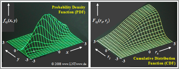
$\text{Example 1:}$ The graphic shows
- the probability density function (left),
- cumulative distribution function (right)
of a two-dimensional Gaussian random variable $(x, y)$ with relatively strong positive correlation of the individual components:
- $$ρ_{xy} = 0.8.$$
As in the $\text{previous examples}$, the random variable is more extended in $x$ direction than in $y$ direction: $σ_x = 2 \cdot σ_y$.
These representations can be interpreted as follows:
- The PDF here is comparable to a mountain ridge extending from the lower left to the upper right.
- The maximum is at $m_x = 0$ and $m_y = 0$. This means that the the two-dimensional random variable is mean-free.
- The 2D–CDF as the integral in two directions over the 2D–PDF increases continuously from lower left to upper right from $0$ to $1$.
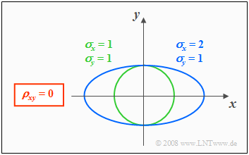
From the conditional equation $f_{xy}(x, y) = \rm const.$ the contour lines of the PDF can be calculated.
If the components $x$ and $y$ are uncorrelated $(ρ_{xy} = 0)$, the equation obtained for the contour lines is:
- $$\frac{x^{\rm 2}}{\sigma_{x}^{\rm 2}}+\frac{y^{\rm 2}}{\sigma_{y}^{\rm 2}} =\rm const.$$
In this case, the contour lines describe the following figures:
- "Circles" $($for $σ_x = σ_y$, green curve$)$, or
- "Ellipses" $($for $σ_x ≠ σ_y$, blue curve$)$ in alignment of the two axes.
More information on this topic with signal examples is provided in the first part "Gaussian random variables without statistical bindings" of the (German language) learning video
- "Gaußsche 2D-Zufallsgrößen" ⇒ "Two-dimensional Gaussian random variables".
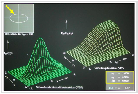
$\text{Example 2:}$
- The graphic shows a snapshot of the first part video "Gaussian random variables without statistical bindings".
- The second video part covers "Gaussian random variables with statistical bindings" according to the following section.
For correlated components $(ρ_{xy} ≠ 0)$ the PDF contour lines are always elliptic, thus also for the special case $σ_x = σ_y$:
- $$f_{xy}(x, y) = {\rm const.} \hspace{0.5cm} \rightarrow \hspace{0.5cm} \frac{x^{\rm 2} }{\sigma_{x}^{\rm 2}}+\frac{y^{\rm 2} }{\sigma_{y}^{\rm 2} }-{\rm 2}\cdot\rho_{xy}\cdot\frac{x\cdot y}{\sigma_x\cdot \sigma_y}={\rm const.}$$
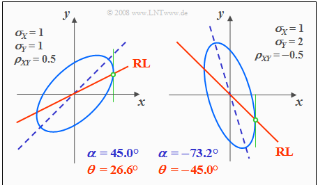
The following graph shows in lighter blue two contour lines for different parameter sets, each with $ρ_{xy} ≠ 0$.
- The ellipse major axis is dashed in dark blue.
- The correlation line or "regression line" $(RL)$ is drawn in solid red.
Based on this plot, the following statements can be made:
- The ellipse shape depends not only on the correlation coefficient $ρ_{xy}$ but also on the ratio of the two standard deviations $σ_x$ and $σ_y$.
- The angle of inclination $α$ of the ellipse major axis (blue dashed straight line) with respect to the $x$–axis also depends on $σ_x$, $σ_y$ and $ρ_{xy}$:
- $$\alpha = {1}/{2} \cdot {\rm arctan } \ ( 2 \cdot \rho_{xy} \cdot \frac {\sigma_x \cdot \sigma_y}{\sigma_x^2 - \sigma_y^2}).$$
- The (red solid) correlation line $y = K(x)$ of a Gaussian random variable always lies below the (blue dashed) ellipse major axis.
- $K(x)$ can also be constructed geometrically from the intersection of the contour lines and their vertical tangents, as indicated in green in the sketches above.
More information on this topic is provided in the (German language) learning video
- "Gaußsche 2D-Zufallsgrößen" ⇒ "Two-dimensional Gaussian random variables".
- Part 1: Gaussian random variables without statistical bindings,
- Part 2: Gaussian random variables with statistical bindings.
Rotation of the coordinate system
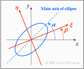
For some tasks it is advantageous to rotate the coordinate system, as indicated in the following graphic:
- The $(ξ, η)$ coordinate system is rotated with respect to the original $(x, y)$ system by the angle $β$.
- In contrast, $α$ denotes the angle between the ellipse major axis and the $x$–axis.
The following relationships exist between the coordinates of the two reference frames:
- $$\xi = \hspace{0.4cm} \cos (\beta) \cdot x + \sin (\beta) \cdot y \hspace{0.55cm}{\rm resp. }\hspace{0.5cm} x = \cos (\beta) \cdot \xi - \sin (\beta) \cdot \eta ,$$
- $$\eta = - \sin (\beta) \cdot x + \cos (\beta) \cdot y \hspace{0.5cm}{\rm resp. }\hspace{0.5cm} y = \sin (\beta) \cdot \xi + \cos (\beta) \cdot \eta .$$
If $(x, y)$ is a Gaussian random variable, then the random variable $(ξ, η)$ is also Gaussian distributed.
Substituting the above equations into the 2D–PDF $f_{xy}(x, y)$ and comparing the coefficients, we obtain the following governing equations for $σ_x$, $σ_y$ and $ρ_{xy}$ respectively $σ_ξ, σ_η$ and $ρ_{ξη}$:
- $$\frac {1}{(1 - \rho_{\xi \eta}^2) \cdot \sigma_\xi^2} = \frac {1}{(1 - \rho_{xy}^2) } \left[ \frac {\cos^2 (\beta)}{\sigma_{x}^2 } + \frac {\sin^2 (\beta)}{\sigma_{y}^2 } - 2 \rho_{xy} \cdot \frac {\sin (\beta) \cdot \cos (\beta)}{\sigma_{x} \cdot \sigma_{y}}\right ] ,$$
- $$\frac {1}{(1 - \rho_{\xi \eta}^2) \cdot \sigma_\eta^2} = \frac {1}{(1 - \rho_{xy}^2) } \left[ \frac {\sin^2 (\beta)}{\sigma_{x}^2 } + \frac {\cos^2 (\beta)}{\sigma_{y}^2 } + 2 \rho_{xy} \cdot \frac {\sin (\beta) \cdot \cos (\beta)}{\sigma_{x} \cdot \sigma_{y}}\right ] ,$$
- $$\frac {\rho_{\xi \eta}}{(1 - \rho_{\xi \eta}^2) \cdot \sigma_\xi\cdot \sigma_\eta}= \frac {1}{(1 - \rho_{xy}^2) } \left[ \frac {\sin (\beta) \cdot \cos (\beta)}{\sigma_{x}^2 } - \frac {\sin (\beta) \cdot \cos (\beta)}{\sigma_{y}^2 } + \frac {\rho_{xy}}{\sigma_{x} \cdot \sigma_{y}} \cdot ( \cos^2( \beta) -\sin^2( \beta)) \right ] .$$
With these three equations, in each case three parameters of the two coordinate systems can be converted directly, which is possible however only in special cases without substantial computational expenditure. Following an example with justifiable computational expenditure.
$\text{Example 3:}$ We consider a two-dimensional Gaussian PDF with the following properties:
- The variances of the two components are equal: $σ_x^2 = σ_y^2 = 1$.
- The correlation coefficient between $x$ and $y$ is $ρ_{xy} = 0.5$.
- The angle of the ellipse major axis with respect to the $x$–axis is thus $α = 45^\circ$.
Notes:
- If the coordinate system were also rotated by $β =45^\circ$, there would be uncorrelated components because of $σ_x = σ_y$ and because of $\sin(β) = \cos(β) = 1/\sqrt{2}$ for the new correlation coefficient ⇒ $ρ_{ξη} = 0$ .
- The two standard deviations – related to the new coordinate system – would then result according to the first two equations to $σ_ξ = \sqrt{1.5}$ and $σ_η = \sqrt{0.5}$.
However, the above sketch is not based on $β = α$ but on $β = α/2$.
With the parameters and equations
- $σ_x = σ_y = 1$, $ρ_{xy} = 0.5$,
- $α = 45^\circ$, $\sin(β) - \cos(β) = \sin(2β)/2 = \sin(α)/2$, and
- $\cos^2(β) - \sin^2(β) = \cos(2β)= \cos(α)$
the system of equations can be represented as follows:
- $${\rm (I)}\hspace{0.8cm}\frac {1}{(1 - \rho_{\xi \eta}^2) \cdot \sigma_\xi^2} = \frac {4}{3} \left[ 1 - \frac {1}{2}\cdot {\sin (\alpha) }\right ] = 0.862 ,$$
- $${\rm (II)}\hspace{0.68cm}\frac {1}{(1 - \rho_{\xi \eta}^2) \cdot \sigma_\eta^2} = \frac {4}{3} \left[ 1 + \frac {1}{2}\cdot {\sin (\alpha) }\right ] = 1.805 ,\hspace{0.28cm}\frac {\rm (I)}{\rm (II)}: \frac {\sigma_\eta}{\sigma_\xi} = \sqrt{\frac{0.862}{1.805} }= 0.691,$$
- $${\rm (III)}\hspace{0.54cm}\frac {\rho_{\xi \eta} }{(1 - \rho_{\xi \eta}^2) \cdot \sigma_\xi\cdot \sigma_\eta}= \frac {\rho_{\xi \eta} }{(1 - \rho_{\xi \eta}^2) \cdot \sigma_\xi^2 \cdot 0.691}=\frac {2}{3}\cdot \cos( \alpha) = 0.471.$$
Dividing now the equation $\rm (III)$ by the equation $\rm (I)$, we get:
- $$ \frac {\rho_{\xi \eta} }{0.691}=\frac {0.471}{0.862}\hspace{0.5cm}\Rightarrow\hspace{0.5cm}{\rho_{\xi \eta} }= 0.378.$$
The other two parameters of the new coordinate system now result in $σ_ξ ≈ 1$ and $σ_η ≈ 0.7$.
Exercises for the chapter
Exercise 4.4: Two-dimensional Gaussian PDF
Exercise 4.4Z: Contour Lines of the "2D-PDF"
Exercise 4.5: Two-dimensional Examination Evaluation
Exercise 4.6: Coordinate Rotation
