Difference between revisions of "Aufgaben:Exercise 4.5: Locality Curve for DSB-AM"
| (10 intermediate revisions by 2 users not shown) | |||
| Line 1: | Line 1: | ||
| − | {{quiz-Header|Buchseite=Signal_Representation/ | + | {{quiz-Header|Buchseite=Signal_Representation/Equivalent Low-Pass Signal and its Spectral Function |
}} | }} | ||
[[File:P_ID751__Sig_A_4_5_neu.png|250px|right|frame|Spectrum of the analytical signal]] | [[File:P_ID751__Sig_A_4_5_neu.png|250px|right|frame|Spectrum of the analytical signal]] | ||
| − | We consider a similar transmission scenario as in [[Aufgaben: | + | We consider a similar transmission scenario as in [[Aufgaben:Exercise_4.4:_Pointer_Diagram_for_DSB-AM|Exrcise 4.4]] (but not the same): |
| − | * | + | * A sinusoidal source signal with amplitude $A_{\rm N} = 2 \ \text{V}$ and frequency $f_{\rm N} = 10 \ \text{kHz}$, |
| − | * | + | *Double-Sideband Amplitude Modulation without carrier suppression with carrier frequency $f_{\rm T} = 50 \ \text{kHz}$. |
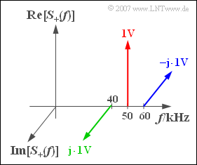
Opposite you see the spectral function $S_+(f)$ of the analytical signal $s_+(t)$. | Opposite you see the spectral function $S_+(f)$ of the analytical signal $s_+(t)$. | ||
| − | When solving, take into account that the equivalent low pass signal is | + | When solving, take into account that the equivalent low-pass signal is in the form |
| − | :$$s_{\rm TP}(t) = a(t) \cdot {\rm e}^{{\rm j}\hspace{0.05cm}\cdot \hspace{0.05cm} \phi(t)} $$ | + | :$$s_{\rm TP}(t) = a(t) \cdot {\rm e}^{{\rm j}\hspace{0.05cm}\cdot \hspace{0.05cm} \phi(t)},\hspace{0.5cm} a(t) ≥ 0.$$ |
| − | + | For $\phi(t)$, the range $–\pi < \phi(t) \leq +\pi$ is permissible and the generally valid equation applies: | |
:$$\phi(t)= {\rm arctan} \hspace{0.1cm}\frac{{\rm Im}\big[s_{\rm | :$$\phi(t)= {\rm arctan} \hspace{0.1cm}\frac{{\rm Im}\big[s_{\rm | ||
TP}(t)\big]}{{\rm Re}\big[s_{\rm TP}(t)\big]}.$$ | TP}(t)\big]}{{\rm Re}\big[s_{\rm TP}(t)\big]}.$$ | ||
| − | |||
| − | |||
| − | |||
| Line 29: | Line 26: | ||
''Hints:'' | ''Hints:'' | ||
| − | *This exercise belongs to the chapter [[Signal_Representation/ | + | *This exercise belongs to the chapter [[Signal_Representation/Equivalent_Low-Pass_Signal_and_its_Spectral_Function|Equivalent Low-Pass Signal and its Spectral Function]]. |
| − | *You can check your solution with the interactive applet [[Applets: | + | *You can check your solution with the interactive applet [[Applets:Physical_Signal_%26_Equivalent_Lowpass_Signal|Physical Signal & Equivalent Low-Pass Signal]] ⇒ "Locality Curve". |
| Line 37: | Line 34: | ||
<quiz display=simple> | <quiz display=simple> | ||
| − | {Calculate the equivalent low pass signal $s_{\rm TP}(t)$ in the frequency and time domain. What is the value of $s_{\rm TP}(t)$ at the start time $t = 0$? | + | {Calculate the equivalent low-pass signal $s_{\rm TP}(t)$ in the frequency and time domain. What is the value of $s_{\rm TP}(t)$ at the start time $t = 0$? |
|type="{}"} | |type="{}"} | ||
$\text{Re}[s_{\text{TP}}(t=0)]\ = \ $ { 1 3% } $\text{V}$ | $\text{Re}[s_{\text{TP}}(t=0)]\ = \ $ { 1 3% } $\text{V}$ | ||
$\text{Im}[s_{\text{TP}}(t=0 )]\ = \ $ { 0. } $\text{V}$ | $\text{Im}[s_{\text{TP}}(t=0 )]\ = \ $ { 0. } $\text{V}$ | ||
| − | {What are the values of $s_{\rm TP}(t)$ at $t = 10 \ {\rm µ} \text{s}= T_0/10$, $t = 25 \ {\rm µ} \text{s}= T_0/4$, $t = 75 \ {\rm µ} \text{s}= 3T_0/4$ and $T_0 = 100 \ {\rm µ} | + | {What are the values of $s_{\rm TP}(t)$ at $t = 10 \ {\rm µ} \text{s}= T_0/10$, $t = 25 \ {\rm µ} \text{s}= T_0/4$, $t = 75 \ {\rm µ} \text{s}= 3T_0/4$ and $T_0 = 100 \ {\rm µs}$? <br>Show that all values are purely real. |
|type="{}"} | |type="{}"} | ||
$\text{Re}[s_{\text{TP}}(t=10 \ {\rm µ} \text{s})]\ = \ $ { 2.176 3% } $\text{V}$ | $\text{Re}[s_{\text{TP}}(t=10 \ {\rm µ} \text{s})]\ = \ $ { 2.176 3% } $\text{V}$ | ||
| Line 49: | Line 46: | ||
$\text{Re}[s_{\text{TP}}(t=100 \ {\rm µ} \text{s})]\ = \ $ { 1 3% } $\text{V}$ | $\text{Re}[s_{\text{TP}}(t=100 \ {\rm µ} \text{s})]\ = \ $ { 1 3% } $\text{V}$ | ||
| − | {What is the magnitude function $a(t)$ | + | {What is the magnitude function $a(t)$ in the time domain? What are the values at times $t = 25 \ {\rm µ} \text{s}$ and $t = 75 \ {\rm µ} \text{s}$? |
|type="{}"} | |type="{}"} | ||
$a(t=25 \ {\rm µ} \text{s})\ = \ $ { 3 3% } $\text{V}$ | $a(t=25 \ {\rm µ} \text{s})\ = \ $ { 3 3% } $\text{V}$ | ||
$a(t=75 \ {\rm µ} \text{s})\ = \ $ { 1 3% } $\text{V}$ | $a(t=75 \ {\rm µ} \text{s})\ = \ $ { 1 3% } $\text{V}$ | ||
| − | {Give the phase function $\phi(t)$ in the time domain | + | {Give the phase function $\phi(t)$ in the time domain. What values result at the times $t = 25 \ {\rm µ} \text{s}$ and $t = 75 \ {\rm µ} \text{s}$? |
|type="{}"} | |type="{}"} | ||
$\phi(t=25 \ {\rm µ} \text{s}) \ = \ $ { 0. } $\text{Grad}$ | $\phi(t=25 \ {\rm µ} \text{s}) \ = \ $ { 0. } $\text{Grad}$ | ||
| Line 66: | Line 63: | ||
{{ML-Kopf}} | {{ML-Kopf}} | ||
| − | [[File:EN_Sig_A_4_5_a.png|250px|right|frame| | + | [[File:EN_Sig_A_4_5_a.png|250px|right|frame|Locality curve at time $t = 0$]] |
| − | '''(1)''' If all | + | '''(1)''' If all Dirac delta lines are shifted to the left by $f_{\rm T} = 50 \ \text{kHz}$ , they are located at $-\hspace{-0.08cm}10 \ \text{kHz}$, $0$ and $+10 \ \text{kHz}$. |
*The equation for $s_{\rm TP}(t)$ is with $\omega_{10} = 2 \pi \cdot 10 \ \text{kHz}$: | *The equation for $s_{\rm TP}(t)$ is with $\omega_{10} = 2 \pi \cdot 10 \ \text{kHz}$: | ||
| Line 94: | Line 91: | ||
{t}/{T_0}) .$$ | {t}/{T_0}) .$$ | ||
| − | *This shows that $s_{\rm TP}(t)$ is real for all times $t$ | + | *This shows that $s_{\rm TP}(t)$ is real for all times $t$. |
| − | * | + | *We obtain for the numerical values we are looking for: |
:$$s_{\rm TP}(t = {\rm 10 \hspace{0.1cm} {\rm µ} s}) = {\rm 1 | :$$s_{\rm TP}(t = {\rm 10 \hspace{0.1cm} {\rm µ} s}) = {\rm 1 | ||
| Line 130: | Line 127: | ||
Re}\left[s_{\rm TP}(t)\right]}$$ | Re}\left[s_{\rm TP}(t)\right]}$$ | ||
| − | Due to the fact that here ${\rm Im}[s_{\rm TP}(t)] = 0$ for all times, one obtains | + | Due to the fact that here ${\rm Im}[s_{\rm TP}(t)] = 0$ for all times, one obtains: |
* If ${\rm Re}[s_{\rm TP}(t)] > 0$ holds, the phase $\phi(t) = 0$. | * If ${\rm Re}[s_{\rm TP}(t)] > 0$ holds, the phase $\phi(t) = 0$. | ||
* On the other hand, if the real part is negative: $\phi(t) = \pi$. | * On the other hand, if the real part is negative: $\phi(t) = \pi$. | ||
| Line 142: | Line 139: | ||
:$$\sin(2 \pi \cdot {t_1}/{T_0}) = -0.5 \hspace{0.3cm} \Rightarrow | :$$\sin(2 \pi \cdot {t_1}/{T_0}) = -0.5 \hspace{0.3cm} \Rightarrow | ||
\hspace{0.3cm} 2 \pi \cdot {t_1}/{T_0} = 2 \pi \cdot | \hspace{0.3cm} 2 \pi \cdot {t_1}/{T_0} = 2 \pi \cdot | ||
| − | {7}/{12}\hspace{0.3cm}{\ | + | {7}/{12}\hspace{0.3cm}{\text{(corresponds to}}\hspace{0.2cm}210^\circ |
)$$ | )$$ | ||
| Line 155: | Line 152: | ||
__NOEDITSECTION__ | __NOEDITSECTION__ | ||
| − | [[Category:Signal Representation: Exercises|^4.3 Equivalent | + | [[Category:Signal Representation: Exercises|^4.3 Equivalent LP Signal and its Spectral Function^]] |
Latest revision as of 14:22, 18 January 2023
We consider a similar transmission scenario as in Exrcise 4.4 (but not the same):
- A sinusoidal source signal with amplitude $A_{\rm N} = 2 \ \text{V}$ and frequency $f_{\rm N} = 10 \ \text{kHz}$,
- Double-Sideband Amplitude Modulation without carrier suppression with carrier frequency $f_{\rm T} = 50 \ \text{kHz}$.
Opposite you see the spectral function $S_+(f)$ of the analytical signal $s_+(t)$.
When solving, take into account that the equivalent low-pass signal is in the form
- $$s_{\rm TP}(t) = a(t) \cdot {\rm e}^{{\rm j}\hspace{0.05cm}\cdot \hspace{0.05cm} \phi(t)},\hspace{0.5cm} a(t) ≥ 0.$$
For $\phi(t)$, the range $–\pi < \phi(t) \leq +\pi$ is permissible and the generally valid equation applies:
- $$\phi(t)= {\rm arctan} \hspace{0.1cm}\frac{{\rm Im}\big[s_{\rm TP}(t)\big]}{{\rm Re}\big[s_{\rm TP}(t)\big]}.$$
Hints:
- This exercise belongs to the chapter Equivalent Low-Pass Signal and its Spectral Function.
- You can check your solution with the interactive applet Physical Signal & Equivalent Low-Pass Signal ⇒ "Locality Curve".
Questions
Solution
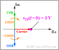
(1) If all Dirac delta lines are shifted to the left by $f_{\rm T} = 50 \ \text{kHz}$ , they are located at $-\hspace{-0.08cm}10 \ \text{kHz}$, $0$ and $+10 \ \text{kHz}$.
- The equation for $s_{\rm TP}(t)$ is with $\omega_{10} = 2 \pi \cdot 10 \ \text{kHz}$:
- $$s_{\rm TP}(t) = {\rm 1 \hspace{0.05cm} V} - {\rm j}\cdot {\rm 1 \hspace{0.05cm} V} \cdot {\rm e}^{{\rm j}\hspace{0.05cm} \omega_{\rm 10} \hspace{0.05cm} t }+{\rm j}\cdot {\rm 1 \hspace{0.05cm} V} \cdot {\rm e}^{-{\rm j}\hspace{0.05cm} \omega_{\rm 10} \hspace{0.05cm} t }$$
- $$\Rightarrow \hspace{0.3cm} s_{\rm TP}(t = 0) = {\rm 1 \hspace{0.05cm} V} - {\rm j}\cdot {\rm 1 \hspace{0.05cm} V} +{\rm j}\cdot {\rm 1 \hspace{0.05cm} V}= {\rm 1 \hspace{0.05cm} V}.$$
- $$\Rightarrow \hspace{0.3cm} {\rm Re}[s_{\rm TP}(t = 0) ] \hspace{0.15 cm}\underline{= {+\rm 1 \hspace{0.05cm} V}}, \hspace{0.2cm}{\rm Im}[s_{\rm TP}(t = 0) ] \hspace{0.15 cm}\underline{= 0} .$$
(2) The above equation can be transformed according to Euler's theorem with $T_0 = 1/f_{\rm N} = 100 \ {\rm µ} \text{s}$ as follows:
- $$\frac{s_{\rm TP}(t)}{{\rm 1 \hspace{0.05cm} V}}\hspace{-0.05cm} =\hspace{-0.05cm}1\hspace{-0.05cm} - \hspace{-0.05cm}{\rm j}\cdot \cos({ \omega_{\rm 10}\hspace{0.05cm} t }) \hspace{-0.05cm}+\hspace{-0.05cm} \sin({ \omega_{\rm 10}\hspace{0.05cm} t }) \hspace{-0.05cm}+\hspace{-0.05cm}{\rm j}\cdot \cos({ \omega_{\rm 10}\hspace{0.05cm} t })\hspace{-0.05cm} + \hspace{-0.05cm} \sin({ \omega_{\rm 10}\hspace{0.05cm} t }) = 1+2 \cdot \sin(2 \pi {t}/{T_0}) .$$
- This shows that $s_{\rm TP}(t)$ is real for all times $t$.
- We obtain for the numerical values we are looking for:
- $$s_{\rm TP}(t = {\rm 10 \hspace{0.1cm} {\rm µ} s}) = {\rm 1 \hspace{0.05cm} V} \cdot \left[1+2 \cdot \sin(36^\circ)\right]\hspace{0.15 cm}\underline{={{\rm +2.176 \hspace{0.05cm} V}}},$$
- $$s_{\rm TP}(t = {\rm 25 \hspace{0.1cm} {\rm µ} s}) = {\rm 1 \hspace{0.05cm} V} \cdot \left[1+2 \cdot \sin(90^\circ)\right]\hspace{0.15 cm}\underline{={{\rm +3 \hspace{0.05cm} V}}},$$
- $$s_{\rm TP}(t = {\rm 75 \hspace{0.1cm} {\rm µ} s}) = {\rm 1 \hspace{0.05cm} V} \cdot \left[1+2 \cdot \sin(270^\circ)\right]\hspace{0.15 cm}\underline{= -{{\rm 1 \hspace{0.05cm} V}}},$$
- $$s_{\rm TP}(t = {\rm 100 \hspace{0.1cm}{\rm µ} s}) = s_{\rm TP}(t = 0) \hspace{0.15 cm}\underline{={{\rm +1 \hspace{0.05cm} V}}}.$$
(3) By definition, $a(t) = |s_{\rm TP}(t)|$. This gives the following numerical values:
- $$a(t = {\rm 25 \hspace{0.1cm} {\rm µ} s}) = s_{\rm TP}(t = {\rm 25 \hspace{0.05cm}{\rm µ} s}) \hspace{0.15 cm}\underline{= {\rm +3 \hspace{0.05cm} V}} , \hspace{4.15 cm}$$
- $$a(t = {\rm 75 \hspace{0.1cm} {\rm µ} s}) = |s_{\rm TP}(t = {\rm 75 \hspace{0.05cm} {\rm µ} s})| \hspace{0.15 cm}\underline{= {\rm +1 \hspace{0.05cm} V}} .$$
(4) In general, the phase function is:
- $$\phi(t)= {\rm arc} \left[s_{\rm TP}(t)\right]= {\rm arctan} \hspace{0.1cm}\frac{{\rm Im}\left[s_{\rm TP}(t)\right]}{{\rm Re}\left[s_{\rm TP}(t)\right]}$$
Due to the fact that here ${\rm Im}[s_{\rm TP}(t)] = 0$ for all times, one obtains:
- If ${\rm Re}[s_{\rm TP}(t)] > 0$ holds, the phase $\phi(t) = 0$.
- On the other hand, if the real part is negative: $\phi(t) = \pi$.
We restrict ourselves here to the time range of one period: $0 \leq t \leq T_0$.
- In the range between $t_1$ and $t_2$ there is a phase of $180^\circ$ otherwise $\text{Re}[s_{\rm TP}(t)] \geq 0$.
- To calculate $t_1$ , the result of subtask (2) can be used:
- $$\sin(2 \pi \cdot {t_1}/{T_0}) = -0.5 \hspace{0.3cm} \Rightarrow \hspace{0.3cm} 2 \pi \cdot {t_1}/{T_0} = 2 \pi \cdot {7}/{12}\hspace{0.3cm}{\text{(corresponds to}}\hspace{0.2cm}210^\circ )$$
- From this one obtains $t_1 = 7/12 · T_0 = 58.33 \ {\rm µ} \text{s}$.
- By similar reasoning one arrives at the result: $t_2 = 11/12 · T_0 = 91.63 \ {\rm µ} \text{s}$.
The values we are looking for are therefore:
- $$\phi(t = 25 \ {\rm µ} \text{s}) \; \underline { = 0},$$
- $$\phi(t = 75 \ {\rm µ} \text{s}) \; \underline { = 180^{\circ}}\; (= \pi).$$

