Difference between revisions of "Aufgaben:Exercise 4.09: Recursive Systematic Convolutional Codes"
| (39 intermediate revisions by 5 users not shown) | |||
| Line 1: | Line 1: | ||
| − | {{quiz-Header|Buchseite= | + | {{quiz-Header|Buchseite=Channel_Coding/The_Basics_of_Turbo_Codes}} |
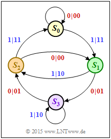
| − | [[File:P_ID3040__KC_A_4_9_v1.png|right|frame| | + | [[File:P_ID3040__KC_A_4_9_v1.png|right|frame|State transition diagram <br>of an RSC code]] |
| − | In | + | In [[Aufgaben:Exercise_4.08:_Repetition_to_the_Convolutional_Codes|$\text{Exercise 4.8}$]] important properties of convolutional codes have already been derived from the state transition diagram, assuming a non-recursive filter structure. |
| − | + | Now a rate $1/2$ RSC code is treated in a similar manner. Here $\rm RSC$ stands for "recursive systematic convolutional". | |
| − | + | The transfer function matrix of an RSC convolutional code can be specified as follows: | |
:$${\boldsymbol{\rm G}}(D) = \left [ 1\hspace{0.05cm},\hspace{0.3cm} G^{(2)}(D)/G^{(1)}(D) \right ] | :$${\boldsymbol{\rm G}}(D) = \left [ 1\hspace{0.05cm},\hspace{0.3cm} G^{(2)}(D)/G^{(1)}(D) \right ] | ||
\hspace{0.05cm}.$$ | \hspace{0.05cm}.$$ | ||
| − | + | Otherwise, exactly the same conditions apply here as in Exercise 4.8. We refer again to the following theory pages: | |
| − | [[ | + | #[[Channel_Coding/Algebraic_and_Polynomial_Description#Systematic_convolutional_codes|"Systematic convolutional codes"]] |
| + | #[[Channel_Coding/Code_Description_with_State_and_Trellis_Diagram#Representation_in_the_state_transition_diagram|"Representation in the state transition diagram"]] | ||
| + | #[[Channel_Coding/Code_Description_with_State_and_Trellis_Diagram#Definition_of_the_free_distance|"Definition of the free distance"]] | ||
| + | #[[Channel_Coding/Algebraic_and_Polynomial_Description#GF.282.29_description_forms_of_a_digital_filter|"GF(2) description forms of a digital filter"]] | ||
| + | #[[Channel_Coding/Algebraic_and_Polynomial_Description#Application_of_the_D.E2.80.93transform_to_rate_.7F.27.22.60UNIQ-MathJax158-QINU.60.22.27.7F_convolution_encoders| "Application of the $D$–transform to rate $1/n$ convolution encoders"]] | ||
| + | #[[Channel_Coding/Algebraic_and_Polynomial_Description#Filter_structure_with_fractional.E2.80.93rational_transfer_function|"Filter structure with fractional–rational transfer function"]] | ||
| − | |||
| − | + | In the state transition diagram, two arrows go from each state. The label is "$u_i \hspace{0.05cm}| \hspace{0.05cm} x_i^{(1)}x_i^{(2)}$". For a systematic code, this involves: | |
| + | * The first code bit is identical to the information bit: $\hspace{0.2cm} x_i^{(1)} = u_i ∈ \{0, \, 1\}$. | ||
| + | * The second code bit is the parity-check bit: $\hspace{0.2cm} x_i^{(2)} = p_i ∈ \{0, \, 1\}$. | ||
| − | |||
| − | |||
| − | |||
| − | |||
| − | |||
| − | |||
| − | |||
| − | |||
| − | |||
| − | |||
| − | |||
| − | |||
| − | |||
| + | <u>Hints:</u> | ||
| + | * The exercise refers to the chapter [[Channel_Coding/The_Basics_of_Turbo_Codes|"Basics of Turbo Codes"]]. | ||
| + | |||
| + | * The following vectorial quantities are used in the questions for this exercise: | ||
| + | :* the information sequence: $\hspace{0.2cm} \underline{u} = (u_1, \, u_2, \text{...} \hspace{0.05cm} )$, | ||
| + | :* the parity-check sequence: $\hspace{0.2cm} \underline{p} = (p_1, \, p_2, \text{...} \hspace{0.05cm})$, | ||
| + | :* the impulse response: $\hspace{0.2cm} \underline{g} = (g_1, \, g_2, \text{...} \hspace{0.05cm} ); \hspace{0.2cm}$ this is equal to the parity sequence $\underline{p}$ for $\underline{u} = (1, \, 0, \, 0, \text{...} \hspace{0.05cm} )$. | ||
| − | === | + | |
| + | |||
| + | ===Questions=== | ||
<quiz display=simple> | <quiz display=simple> | ||
| − | { | + | {What is the impulse response $\underline{g}$ ? |
| + | |type="()"} | ||
| + | + $\underline{g} = (1, \, 1, \, 1, \, 0, \, 1, \, 1, \, 0, \, 1, \, 1, \text{...} \hspace{0.05cm})$. | ||
| + | - $\underline{g} = (1, \, 0, \, 1, \, 0, \, 0, \, 0, \, 0, \, 0, \, 0, \text{...} \hspace{0.05cm})$. | ||
| + | |||
| + | {It holds $\underline{u} = (1, \, 1, \, 0, \, 1)$. Which statements hold for the parity sequence $\underline{p}$ ? | ||
|type="[]"} | |type="[]"} | ||
| − | + | + | - $\underline{p} = (1, \, 0, \, 1, \, 0, \, 0, \, 0, \, 0, \, 0, \, 0, \, 0, \, 0, \, 0, \text{...} \hspace{0.05cm})$. |
| − | - | + | + $\underline{p} = (1, \, 0, \, 0, \, 0, \, 0, \, 1, \, 1, \, 0, \, 1, \, 1, \, 0, \, 1, \text{...} \hspace{0.05cm})$. |
| + | - With limited information sequence $\underline{u}$ ⇒ $\underline{p}$ is also limited. | ||
| − | { | + | {What is the $D$–transfer function $G(D)$? |
| + | |type="[]"} | ||
| + | + $G(D) = 1 + D + D^2 + D^4 + D^5 + D^7 + D^8 + \text{...} \hspace{0.05cm}$. | ||
| + | + $G(D) = (1 + D^2)/(1 + D + D^2)$. | ||
| + | - $G(D) = (1 + D + D^2)/(1 + D^2)$. | ||
| + | |||
| + | {Now let $\underline{u} = (1, \, 1, \, 1)$. Which statements hold for the parity sequence $\underline{p}$? | ||
| + | |type="[]"} | ||
| + | + $\underline{p} = (1, \, 0, \, 1, \, 0, \, 0, \, 0, \, 0, \, 0, \, 0, \, 0, \, 0, \, 0, \text{...} \hspace{0.05cm})$. | ||
| + | - $\underline{p} = (1, \, 0, \, 0, \, 0, \, 0, \, 1, \, 1, \, 0, \, 1, \, 1, \, 0, \, 1, \text{...} \hspace{0.05cm})$. | ||
| + | - With limited information sequence $\underline{u}$ ⇒ $\underline{p}$ is also limited. | ||
| + | |||
| + | {What is the free distance $d_{\rm F}$ of this RSC encoder? | ||
|type="{}"} | |type="{}"} | ||
| − | $ | + | $d_{\rm F} \ = \ ${ 5 3% } |
</quiz> | </quiz> | ||
| − | === | + | ===Solution=== |
{{ML-Kopf}} | {{ML-Kopf}} | ||
| − | '''(1)''' | + | '''(1)''' Tracing the transitions in the state diagram for the sequence $\underline{u} = (1, \, 0, \, 0, \, 0, \, 0, \, 0, \, 0, \, 0, \, 0)$ at the input, we get the path |
| − | '''(2)''' | + | :$$S_0 → S_1 → S_3 → S_2 → S_1 → S_3 → S_2 → S_1 → S_3 → \hspace{0.05cm}\text{...} \hspace{0.05cm}$$ |
| − | '''(3)''' | + | |
| − | '''(4)''' | + | *For each transition, the first code symbol $x_i^{(1)}$ is equal to the information bit $u_i$ and the code symbol $x_i^{(2)}$ indicates the parity-check bit $p_i$. |
| − | '''(5)''' | + | |
| + | *This gives the result corresponding to <u>solution proposition 1</u>: | ||
| + | :$$\underline{p}= (\hspace{0.05cm}1\hspace{0.05cm}, | ||
| + | \hspace{0.05cm}1\hspace{0.05cm}, | ||
| + | \hspace{0.05cm}1\hspace{0.05cm}, | ||
| + | \hspace{0.05cm} 0\hspace{0.05cm}, | ||
| + | \hspace{0.05cm} 1\hspace{0.05cm}, | ||
| + | \hspace{0.05cm} 1\hspace{0.05cm}, | ||
| + | \hspace{0.05cm} 0\hspace{0.05cm}, | ||
| + | \hspace{0.05cm} 1\hspace{0.05cm}, | ||
| + | \hspace{0.05cm} 1\hspace{0.05cm},\hspace{0.05cm}\text{...} \hspace{0.05cm}) | ||
| + | = \underline{g}\hspace{0.05cm}.$$ | ||
| + | |||
| + | *For any RSC code, the impulse response $\underline{g}$ is infinite in length and becomes periodic at some point, in this example with period $P = 3$ and "$0, \, 1, \, 1$". | ||
| + | |||
| + | |||
| + | |||
| + | [[File:EN_KC_A_4_9b_v1.png|right|frame|Clarification of $\underline{p} = (1, \, 1, \, 0, \, 1)^{\rm T} \cdot \mathbf{G}$]] | ||
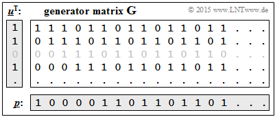
| + | '''(2)''' The graph shows the solution of this exercise according to the equation $\underline{p} = \underline{u}^{\rm T} \cdot \mathbf{G}$. | ||
| + | * Here the generator matrix $\mathbf{G}$ is infinitely extended downward and to the right. | ||
| + | |||
| + | *The correct solution is <u>proposal 2</u>. | ||
| + | |||
| + | |||
| + | |||
| + | '''(3)''' Correct are <u>the proposed solutions 1 and 2</u>: | ||
| + | *Between the impulse response $\underline{g}$ and the $D$–transfer function $\mathbf{G}(D)$ there is the relation according to the first proposed solution: | ||
| + | :$$\underline{g}= (\hspace{-0.05cm}1\hspace{-0.05cm}, | ||
| + | \hspace{-0.07cm}1\hspace{-0.07cm}, | ||
| + | \hspace{-0.07cm}1\hspace{-0.07cm}, | ||
| + | \hspace{-0.07cm}0\hspace{-0.07cm}, | ||
| + | \hspace{-0.07cm}1\hspace{-0.07cm}, | ||
| + | \hspace{-0.07cm}1\hspace{-0.07cm}, | ||
| + | \hspace{-0.07cm}0\hspace{-0.07cm}, | ||
| + | \hspace{-0.07cm}1\hspace{-0.07cm}, | ||
| + | \hspace{-0.07cm}1\hspace{-0.07cm}, | ||
| + | ... ) \hspace{0.3cm} \circ\!\!-\!\!\!-^{\hspace{-0.25cm}D}\!\!\!-\!\!\bullet \hspace{0.3cm} | ||
| + | G(D) = 1\hspace{-0.05cm}+\hspace{-0.05cm} D\hspace{-0.05cm} +\hspace{-0.05cm} D^2\hspace{-0.05cm} +\hspace{-0.05cm} D^4 \hspace{-0.05cm}+\hspace{-0.05cm} D^5 \hspace{-0.05cm}+\hspace{-0.05cm} D^7 \hspace{-0.05cm}+\hspace{-0.05cm} D^8 + \text{...} .$$ | ||
| + | |||
| + | *Let us now examine the second proposal: | ||
| + | :$$G(D) = \frac{1+ D^2}{1+ D + D^2} \hspace{0.3cm}\Rightarrow \hspace{0.3cm} | ||
| + | G(D) \cdot [1+ D + D^2] = 1+ D^2 \hspace{0.05cm}.$$ | ||
| + | |||
| + | *The following calculation shows that this equation is indeed true: | ||
| + | :$$(1+ D+ D^2+ D^4 +D^5 + D^7 + D^8 + \hspace{0.05cm} \text{...}) \cdot (1+ D+ D^2 ) =$$ | ||
| + | :$$=1+ D+ D^2\hspace{1.05cm} +D^4 + D^5 \hspace{1.05cm} +D^7 + D^8 \hspace{1.05cm} + D^{10}+ \hspace{0.05cm} \text{...}$$ | ||
| + | :$$+ \hspace{0.8cm}D+ D^2+D^3 \hspace{1.05cm}+ D^5 + D^6 \hspace{1.05cm} +D^8 + D^9 \hspace{1.25cm} +\hspace{0.05cm} \text{...} $$ | ||
| + | :$$+ \hspace{1.63cm} D^2+D^3+ D^4 \hspace{1.05cm}+ D^6 +D^7 \hspace{1.05cm}+ D^9 + D^{10} \hspace{0.12cm}+ \hspace{0.05cm} \text{...}$$ | ||
| + | :$$=\underline{1\hspace{0.72 | ||
| + | cm}+ D^2} \hspace{0.05cm}.$$ | ||
| + | |||
| + | *But since equation '''(2)''' is true, the last equation must be false. | ||
| + | |||
| + | |||
| + | |||
| + | '''(4)''' Correct is only the <u>proposed solution 1</u>: | ||
| + | *From $\underline{u} = (1, \, 1, \, 1)$ follows $U(D) = 1 + D + D^2$. Thus also holds: | ||
| + | :$$P(D) = U(D) \cdot G(D) = (1+D+D^2) \cdot \frac{1+D^2}{1+D+D^2}= 1+D^2\hspace{0.3cm} | ||
| + | \Rightarrow\hspace{0.3cm} \underline{p}= (\hspace{0.05cm}1\hspace{0.05cm},\hspace{0.05cm} 0\hspace{0.05cm},\hspace{0.05cm} 1\hspace{0.05cm},\hspace{0.05cm} 0\hspace{0.05cm},\hspace{0.05cm} 0\hspace{0.05cm},\hspace{0.05cm}\text{...}\hspace{0.05cm})\hspace{0.05cm}. $$ | ||
| + | * If the variables $u_i$ and $g_i$ were real-valued, the $($discrete$)$ convolution $\underline{p} = \underline{u} * \underline{g} $ would always lead to a broadening. | ||
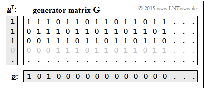
| + | [[File:EN_KC_A_4_9d_v1.png|right|frame|Clarification of $\underline{p} = (1, \, 1, \, 1, \, 0, \, ...)^{\rm T} \cdot \mathbf{G}$]] | ||
| + | *In this case $\underline{p}$ would be broader than $\underline{u}$ and also broader than $\underline{g}$. | ||
| + | |||
| + | * On the other hand, for $u_i ∈ {\rm GF}(2)$ and $g_i ∈ {\rm GF}(2)$ it may $($but need not$)$ happen that even with unlimited $\underline{u}$ or for unlimited $\underline{g}$ the convolution product $\underline{p} = \underline{u} * \underline{g}$ is limited. | ||
| + | |||
| + | *The result is finally checked according to the equation $\underline{p} = \underline{u}^{\rm T} \cdot \mathbf{G}$ is checked. See graph on the right. | ||
| + | |||
| + | |||
| + | |||
| + | '''(5)''' Following a similar procedure as in [[Aufgaben:Exercise_4.08:_Repetition_to_the_Convolutional_Codes|$\text{Exercise A4.8}$, (4)]], one can see: | ||
| + | *The free distance is again determined by the path | ||
| + | :$$S_0 → S_0 → S_1 → S_2 → S_0 → S_0 → \hspace{0.05cm}\text{...}\hspace{0.05cm}.$$ | ||
| + | *But the associated encoded sequence $\underline{x}$ is now " $00 \ 11 \ 10 \ 11 \ 00 \ ... $". | ||
| + | |||
| + | *This gives the free distance to $d_{\rm F} \ \underline{= 5}$. | ||
| + | |||
| + | *In contrast, in the non-recursive code $($Exercise 4.8$)$, the free distance was $d_{\rm F} = 3$. | ||
{{ML-Fuß}} | {{ML-Fuß}} | ||
| − | [[Category: | + | [[Category:Channel Coding: Exercises|^4.3 About the Turbo Codes^]] |
Latest revision as of 18:06, 13 March 2023
In $\text{Exercise 4.8}$ important properties of convolutional codes have already been derived from the state transition diagram, assuming a non-recursive filter structure.
Now a rate $1/2$ RSC code is treated in a similar manner. Here $\rm RSC$ stands for "recursive systematic convolutional".
The transfer function matrix of an RSC convolutional code can be specified as follows:
- $${\boldsymbol{\rm G}}(D) = \left [ 1\hspace{0.05cm},\hspace{0.3cm} G^{(2)}(D)/G^{(1)}(D) \right ] \hspace{0.05cm}.$$
Otherwise, exactly the same conditions apply here as in Exercise 4.8. We refer again to the following theory pages:
- "Systematic convolutional codes"
- "Representation in the state transition diagram"
- "Definition of the free distance"
- "GF(2) description forms of a digital filter"
- "Application of the $D$–transform to rate $1/n$ convolution encoders"
- "Filter structure with fractional–rational transfer function"
In the state transition diagram, two arrows go from each state. The label is "$u_i \hspace{0.05cm}| \hspace{0.05cm} x_i^{(1)}x_i^{(2)}$". For a systematic code, this involves:
- The first code bit is identical to the information bit: $\hspace{0.2cm} x_i^{(1)} = u_i ∈ \{0, \, 1\}$.
- The second code bit is the parity-check bit: $\hspace{0.2cm} x_i^{(2)} = p_i ∈ \{0, \, 1\}$.
Hints:
- The exercise refers to the chapter "Basics of Turbo Codes".
- The following vectorial quantities are used in the questions for this exercise:
- the information sequence: $\hspace{0.2cm} \underline{u} = (u_1, \, u_2, \text{...} \hspace{0.05cm} )$,
- the parity-check sequence: $\hspace{0.2cm} \underline{p} = (p_1, \, p_2, \text{...} \hspace{0.05cm})$,
- the impulse response: $\hspace{0.2cm} \underline{g} = (g_1, \, g_2, \text{...} \hspace{0.05cm} ); \hspace{0.2cm}$ this is equal to the parity sequence $\underline{p}$ for $\underline{u} = (1, \, 0, \, 0, \text{...} \hspace{0.05cm} )$.
Questions
Solution
- $$S_0 → S_1 → S_3 → S_2 → S_1 → S_3 → S_2 → S_1 → S_3 → \hspace{0.05cm}\text{...} \hspace{0.05cm}$$
- For each transition, the first code symbol $x_i^{(1)}$ is equal to the information bit $u_i$ and the code symbol $x_i^{(2)}$ indicates the parity-check bit $p_i$.
- This gives the result corresponding to solution proposition 1:
- $$\underline{p}= (\hspace{0.05cm}1\hspace{0.05cm}, \hspace{0.05cm}1\hspace{0.05cm}, \hspace{0.05cm}1\hspace{0.05cm}, \hspace{0.05cm} 0\hspace{0.05cm}, \hspace{0.05cm} 1\hspace{0.05cm}, \hspace{0.05cm} 1\hspace{0.05cm}, \hspace{0.05cm} 0\hspace{0.05cm}, \hspace{0.05cm} 1\hspace{0.05cm}, \hspace{0.05cm} 1\hspace{0.05cm},\hspace{0.05cm}\text{...} \hspace{0.05cm}) = \underline{g}\hspace{0.05cm}.$$
- For any RSC code, the impulse response $\underline{g}$ is infinite in length and becomes periodic at some point, in this example with period $P = 3$ and "$0, \, 1, \, 1$".
(2) The graph shows the solution of this exercise according to the equation $\underline{p} = \underline{u}^{\rm T} \cdot \mathbf{G}$.
- Here the generator matrix $\mathbf{G}$ is infinitely extended downward and to the right.
- The correct solution is proposal 2.
(3) Correct are the proposed solutions 1 and 2:
- Between the impulse response $\underline{g}$ and the $D$–transfer function $\mathbf{G}(D)$ there is the relation according to the first proposed solution:
- $$\underline{g}= (\hspace{-0.05cm}1\hspace{-0.05cm}, \hspace{-0.07cm}1\hspace{-0.07cm}, \hspace{-0.07cm}1\hspace{-0.07cm}, \hspace{-0.07cm}0\hspace{-0.07cm}, \hspace{-0.07cm}1\hspace{-0.07cm}, \hspace{-0.07cm}1\hspace{-0.07cm}, \hspace{-0.07cm}0\hspace{-0.07cm}, \hspace{-0.07cm}1\hspace{-0.07cm}, \hspace{-0.07cm}1\hspace{-0.07cm}, ... ) \hspace{0.3cm} \circ\!\!-\!\!\!-^{\hspace{-0.25cm}D}\!\!\!-\!\!\bullet \hspace{0.3cm} G(D) = 1\hspace{-0.05cm}+\hspace{-0.05cm} D\hspace{-0.05cm} +\hspace{-0.05cm} D^2\hspace{-0.05cm} +\hspace{-0.05cm} D^4 \hspace{-0.05cm}+\hspace{-0.05cm} D^5 \hspace{-0.05cm}+\hspace{-0.05cm} D^7 \hspace{-0.05cm}+\hspace{-0.05cm} D^8 + \text{...} .$$
- Let us now examine the second proposal:
- $$G(D) = \frac{1+ D^2}{1+ D + D^2} \hspace{0.3cm}\Rightarrow \hspace{0.3cm} G(D) \cdot [1+ D + D^2] = 1+ D^2 \hspace{0.05cm}.$$
- The following calculation shows that this equation is indeed true:
- $$(1+ D+ D^2+ D^4 +D^5 + D^7 + D^8 + \hspace{0.05cm} \text{...}) \cdot (1+ D+ D^2 ) =$$
- $$=1+ D+ D^2\hspace{1.05cm} +D^4 + D^5 \hspace{1.05cm} +D^7 + D^8 \hspace{1.05cm} + D^{10}+ \hspace{0.05cm} \text{...}$$
- $$+ \hspace{0.8cm}D+ D^2+D^3 \hspace{1.05cm}+ D^5 + D^6 \hspace{1.05cm} +D^8 + D^9 \hspace{1.25cm} +\hspace{0.05cm} \text{...} $$
- $$+ \hspace{1.63cm} D^2+D^3+ D^4 \hspace{1.05cm}+ D^6 +D^7 \hspace{1.05cm}+ D^9 + D^{10} \hspace{0.12cm}+ \hspace{0.05cm} \text{...}$$
- $$=\underline{1\hspace{0.72 cm}+ D^2} \hspace{0.05cm}.$$
- But since equation (2) is true, the last equation must be false.
(4) Correct is only the proposed solution 1:
- From $\underline{u} = (1, \, 1, \, 1)$ follows $U(D) = 1 + D + D^2$. Thus also holds:
- $$P(D) = U(D) \cdot G(D) = (1+D+D^2) \cdot \frac{1+D^2}{1+D+D^2}= 1+D^2\hspace{0.3cm} \Rightarrow\hspace{0.3cm} \underline{p}= (\hspace{0.05cm}1\hspace{0.05cm},\hspace{0.05cm} 0\hspace{0.05cm},\hspace{0.05cm} 1\hspace{0.05cm},\hspace{0.05cm} 0\hspace{0.05cm},\hspace{0.05cm} 0\hspace{0.05cm},\hspace{0.05cm}\text{...}\hspace{0.05cm})\hspace{0.05cm}. $$
- If the variables $u_i$ and $g_i$ were real-valued, the $($discrete$)$ convolution $\underline{p} = \underline{u} * \underline{g} $ would always lead to a broadening.
- In this case $\underline{p}$ would be broader than $\underline{u}$ and also broader than $\underline{g}$.
- On the other hand, for $u_i ∈ {\rm GF}(2)$ and $g_i ∈ {\rm GF}(2)$ it may $($but need not$)$ happen that even with unlimited $\underline{u}$ or for unlimited $\underline{g}$ the convolution product $\underline{p} = \underline{u} * \underline{g}$ is limited.
- The result is finally checked according to the equation $\underline{p} = \underline{u}^{\rm T} \cdot \mathbf{G}$ is checked. See graph on the right.
(5) Following a similar procedure as in $\text{Exercise A4.8}$, (4), one can see:
- The free distance is again determined by the path
- $$S_0 → S_0 → S_1 → S_2 → S_0 → S_0 → \hspace{0.05cm}\text{...}\hspace{0.05cm}.$$
- But the associated encoded sequence $\underline{x}$ is now " $00 \ 11 \ 10 \ 11 \ 00 \ ... $".
- This gives the free distance to $d_{\rm F} \ \underline{= 5}$.
- In contrast, in the non-recursive code $($Exercise 4.8$)$, the free distance was $d_{\rm F} = 3$.


