Difference between revisions of "Applets:Coherent and Non-Coherent On-Off Keying"
| (5 intermediate revisions by 2 users not shown) | |||
| Line 11: | Line 11: | ||
| − | The applet returns the | + | The applet returns the joint probabilities ${\rm Pr}(\boldsymbol{r_0} \cap \boldsymbol{s_1})$ ⇒ $($filled blue area in the PDF graph$)$ and ${\rm Pr}(\boldsymbol{r_1} \cap \boldsymbol{s_0})$ ⇒ $($red area$)$ and as a final result: |
:$$p_{\rm S} = {\rm Pr}(\boldsymbol{r} \ne \boldsymbol{s})= {\rm Pr}(\boldsymbol{r_0} \cap \boldsymbol{s_1}) + {\rm Pr}(\boldsymbol{r_1} \cap \boldsymbol{s_0}). $$ | :$$p_{\rm S} = {\rm Pr}(\boldsymbol{r} \ne \boldsymbol{s})= {\rm Pr}(\boldsymbol{r_0} \cap \boldsymbol{s_1}) + {\rm Pr}(\boldsymbol{r_1} \cap \boldsymbol{s_0}). $$ | ||
*All these quantities also depend on the decision threshold $G$ whose optimal value in each case is also determined. | *All these quantities also depend on the decision threshold $G$ whose optimal value in each case is also determined. | ||
| Line 34: | Line 34: | ||
*With coherent demodulation, the signal space constellation of the received signal is equal to that of the transmitted signal and again consists of the two points $\boldsymbol{r}_0=\boldsymbol{s}_0$ and $\boldsymbol{r}_1=\boldsymbol{s}_1$. | *With coherent demodulation, the signal space constellation of the received signal is equal to that of the transmitted signal and again consists of the two points $\boldsymbol{r}_0=\boldsymbol{s}_0$ and $\boldsymbol{r}_1=\boldsymbol{s}_1$. | ||
| − | *In this case, the AWGN noise is one-dimensional with variance $\sigma_{\rm AWGN}^2$ and one obtains corresponding to the [[Digital_Signal_Transmission/Approximation_of_the_Error_Probability#Error_probability_for_symbols_with_equal_probability|"theory | + | *In this case, the AWGN noise is one-dimensional with variance $\sigma_{\rm AWGN}^2$ and one obtains corresponding to the [[Digital_Signal_Transmission/Approximation_of_the_Error_Probability#Error_probability_for_symbols_with_equal_probability|"theory section"]] for the "symbol error probability": |
:$$p_{\rm S} = {\rm Pr}(\boldsymbol{r}\ne \boldsymbol{s})= {\rm Q} \left ( \frac{s_0/2}{\sigma_{\rm AWGN}}\right ) | :$$p_{\rm S} = {\rm Pr}(\boldsymbol{r}\ne \boldsymbol{s})= {\rm Q} \left ( \frac{s_0/2}{\sigma_{\rm AWGN}}\right ) | ||
= {\rm Q} \left ( \sqrt{ {E_{\rm S}}/{N_0}}\right ) \hspace{0.05cm}. $$ | = {\rm Q} \left ( \sqrt{ {E_{\rm S}}/{N_0}}\right ) \hspace{0.05cm}. $$ | ||
| Line 67: | Line 67: | ||
===On–Off–Keying with noncoherent demodulation=== | ===On–Off–Keying with noncoherent demodulation=== | ||
| − | The following diagram shows the structure $($in the equivalent low-pass range$)$ of the optimal OOK receiver for incoherent demodulation. See [[Digital_Signal_Transmission/Carrier_Frequency_Systems_with_Non-Coherent_Demodulation#Non-coherent_demodulation_of_.22on.E2.80.93off_keying.22_.28OOK.29|Detailed description]]. According to this graph applies: | + | The following diagram shows the structure $($in the equivalent low-pass range$)$ of the optimal OOK receiver for incoherent demodulation. See [[Digital_Signal_Transmission/Carrier_Frequency_Systems_with_Non-Coherent_Demodulation#Non-coherent_demodulation_of_.22on.E2.80.93off_keying.22_.28OOK.29|"Detailed description"]]. According to this graph applies: |
[[File:EN_Dig_T_4_5_S2b_neu.png|right|frame|Receiver for incoherent OOK demodulation $($complex signals are labeled blue$)$|class=fit]] | [[File:EN_Dig_T_4_5_S2b_neu.png|right|frame|Receiver for incoherent OOK demodulation $($complex signals are labeled blue$)$|class=fit]] | ||
| Line 73: | Line 73: | ||
*The input signal $\boldsymbol{r}(t) = \boldsymbol{s}(t) \cdot {\rm e}^{\hspace{0.02cm}{\rm j}\hspace{0.03cm}\phi} + \boldsymbol{n}(t)$ at the receiver is generally complex because of the current phase angle $\phi$ and because of the complex noise term $\boldsymbol{n}(t)$. | *The input signal $\boldsymbol{r}(t) = \boldsymbol{s}(t) \cdot {\rm e}^{\hspace{0.02cm}{\rm j}\hspace{0.03cm}\phi} + \boldsymbol{n}(t)$ at the receiver is generally complex because of the current phase angle $\phi$ and because of the complex noise term $\boldsymbol{n}(t)$. | ||
| − | *Now the correlation between the complex received signal $\boldsymbol{r}(t)$ and a [[Digital_Signal_Transmission/Signals,_Basis_Functions_and_Vector_Spaces#Basis_functions_of_complex_time_signals| complex basis function]] $\boldsymbol{\xi}(t)$ is required.<br> | + | *Now the correlation between the complex received signal $\boldsymbol{r}(t)$ and a [[Digital_Signal_Transmission/Signals,_Basis_Functions_and_Vector_Spaces#Basis_functions_of_complex_time_signals|"complex basis function"]] $\boldsymbol{\xi}(t)$ is required.<br> |
*The result is the $($complex$)$ detected value $\boldsymbol{r}$, from which the magnitude $y = |\boldsymbol{r}(t)|$ is formed as a real decision input.<br> | *The result is the $($complex$)$ detected value $\boldsymbol{r}$, from which the magnitude $y = |\boldsymbol{r}(t)|$ is formed as a real decision input.<br> | ||
| Line 79: | Line 79: | ||
*If $y \gt G$, then the estimated value $m_0$ for the symbol $\boldsymbol{s}_{0}$ is output, otherwise the estimated value $m_1$ for the symbol $\boldsymbol{s}_{1}$. | *If $y \gt G$, then the estimated value $m_0$ for the symbol $\boldsymbol{s}_{0}$ is output, otherwise the estimated value $m_1$ for the symbol $\boldsymbol{s}_{1}$. | ||
| − | *Once again, the mean symbol error probability can be represented as the sum of two | + | *Once again, the mean symbol error probability can be represented as the sum of two joint probabilities: |
:$$p_{\rm S} = {\rm Pr}(\boldsymbol{r}\ne \boldsymbol{s}) = {\rm Pr}(\boldsymbol{r_0} \cap \boldsymbol{s_1}) | :$$p_{\rm S} = {\rm Pr}(\boldsymbol{r}\ne \boldsymbol{s}) = {\rm Pr}(\boldsymbol{r_0} \cap \boldsymbol{s_1}) | ||
+ {\rm Pr}(\boldsymbol{r_1} \cap \boldsymbol{s_0}).$$ | + {\rm Pr}(\boldsymbol{r_1} \cap \boldsymbol{s_0}).$$ | ||
| Line 99: | Line 99: | ||
$\rm Rayleigh\ portion$<br> | $\rm Rayleigh\ portion$<br> | ||
| − | Considering the AWGN–noise, $\boldsymbol{r_1}=\boldsymbol{s_1} + \boldsymbol{n_1}$. The noise component $\boldsymbol{n_1}$ has a [[Theory_of_Stochastic_Signals/Further_Distributions#Rayleigh_PDF|Rayleigh distribution]] $($amount of the two mean-free Gaussian components for $I$ and $Q)$. | + | Considering the AWGN–noise, $\boldsymbol{r_1}=\boldsymbol{s_1} + \boldsymbol{n_1}$. The noise component $\boldsymbol{n_1}$ has a [[Theory_of_Stochastic_Signals/Further_Distributions#Rayleigh_PDF|"Rayleigh distribution"]] $($amount of the two mean-free Gaussian components for $I$ and $Q)$. |
*Their conditional PDF is with the rotationally symmetric noise component $\eta$ with $\sigma=\sigma_{\rm AWGN}$ : | *Their conditional PDF is with the rotationally symmetric noise component $\eta$ with $\sigma=\sigma_{\rm AWGN}$ : | ||
| Line 106: | Line 106: | ||
:$${\rm Pr}(\boldsymbol{r_0}|\boldsymbol{s_1}) = \int_{G}^{\infty}f_{\rm Rayleigh}(\eta) \,{\rm d} \eta | :$${\rm Pr}(\boldsymbol{r_0}|\boldsymbol{s_1}) = \int_{G}^{\infty}f_{\rm Rayleigh}(\eta) \,{\rm d} \eta | ||
\hspace{0.05cm},$$ | \hspace{0.05cm},$$ | ||
| − | :and with the factor $1/2$ because of the equally probable | + | :and with the factor $1/2$ because of the equally probable transmitted symbols, the joint probability: |
:$${\rm Pr}(\boldsymbol{r_0} \cap \boldsymbol{s_1}) = 1/2 \cdot {\rm Pr}(\boldsymbol{r_0}|\boldsymbol{s_1})= 1/2 \cdot \int_{G}^{\infty}f_{\rm Rayleigh}(\eta) \,{\rm d} \eta | :$${\rm Pr}(\boldsymbol{r_0} \cap \boldsymbol{s_1}) = 1/2 \cdot {\rm Pr}(\boldsymbol{r_0}|\boldsymbol{s_1})= 1/2 \cdot \int_{G}^{\infty}f_{\rm Rayleigh}(\eta) \,{\rm d} \eta | ||
\hspace{0.05cm}.$$ | \hspace{0.05cm}.$$ | ||
| Line 112: | Line 112: | ||
$\rm Rice\ portion$<br> | $\rm Rice\ portion$<br> | ||
| − | The noise component $\boldsymbol{n_0}$ has a [[Theory_of_Stochastic_Signals/Further_Distributions#Rice_PDF|Rice distribution]] | + | The noise component $\boldsymbol{n_0}$ has a [[Theory_of_Stochastic_Signals/Further_Distributions#Rice_PDF|"Rice distribution"]] |
$($magnitude of Gaussian components with mean values $m_x$ and $m_y)$ ⇒ constant $C=\sqrt{m_x^2 + m_y^2}$<br>$($Note: In the applet, the constant $C$ is denoted by $C_{\rm Rice}$ $)$. | $($magnitude of Gaussian components with mean values $m_x$ and $m_y)$ ⇒ constant $C=\sqrt{m_x^2 + m_y^2}$<br>$($Note: In the applet, the constant $C$ is denoted by $C_{\rm Rice}$ $)$. | ||
:$$f_{y\hspace{0.05cm}\vert \hspace{0.05cm}\boldsymbol{s_0}} (\eta \hspace{0.05cm}\vert \hspace{0.05cm} \boldsymbol{s_0})=\frac{\eta}{\sigma^2}\cdot{\rm e}^{-({C^2+\it \eta^{\rm 2} })/ ({\rm 2 \it \sigma^{\rm 2} })}\cdot {\rm I_0}(\frac{\it \eta\cdot C}{\sigma^{\rm 2} }) = f_{\rm Rice}(\eta) \hspace{1.4cm}{\rm with} \hspace{1.4cm} {\rm I_0}(\eta) = \sum_{k=0}^{\infty}\frac{(\eta/2)^{2k} }{k! \cdot {\rm \Gamma ({\it k}+1)} }.$$ | :$$f_{y\hspace{0.05cm}\vert \hspace{0.05cm}\boldsymbol{s_0}} (\eta \hspace{0.05cm}\vert \hspace{0.05cm} \boldsymbol{s_0})=\frac{\eta}{\sigma^2}\cdot{\rm e}^{-({C^2+\it \eta^{\rm 2} })/ ({\rm 2 \it \sigma^{\rm 2} })}\cdot {\rm I_0}(\frac{\it \eta\cdot C}{\sigma^{\rm 2} }) = f_{\rm Rice}(\eta) \hspace{1.4cm}{\rm with} \hspace{1.4cm} {\rm I_0}(\eta) = \sum_{k=0}^{\infty}\frac{(\eta/2)^{2k} }{k! \cdot {\rm \Gamma ({\it k}+1)} }.$$ | ||
| − | This gives the second | + | This gives the second joint probability: |
:$${\rm Pr}(\boldsymbol{r_1} \cap \boldsymbol{s_0}) = 1/2 \cdot \int_{0}^{G}f_{\rm Rice}(\eta) \,{\rm d} \eta | :$${\rm Pr}(\boldsymbol{r_1} \cap \boldsymbol{s_0}) = 1/2 \cdot \int_{0}^{G}f_{\rm Rice}(\eta) \,{\rm d} \eta | ||
| Line 129: | Line 129: | ||
:$$p_{\rm S} = {\rm Pr}(\boldsymbol{r}\ne \boldsymbol{s}) = {\rm Pr}(\boldsymbol{r_0} \cap \boldsymbol{s_1}) | :$$p_{\rm S} = {\rm Pr}(\boldsymbol{r}\ne \boldsymbol{s}) = {\rm Pr}(\boldsymbol{r_0} \cap \boldsymbol{s_1}) | ||
+ {\rm Pr}(\boldsymbol{r_1} \cap \boldsymbol{s_0}).$$ | + {\rm Pr}(\boldsymbol{r_1} \cap \boldsymbol{s_0}).$$ | ||
| − | *The area marked in blue gives the | + | *The area marked in blue gives the joint probability ${\rm Pr}(\boldsymbol{r_0} \cap \boldsymbol{s_1}) \approx 2.2\%$ This is calculated as the integral over half the Rayleigh PDF in the range from $G$ to $\infty$. |
| − | *The red highlighted area gives the | + | *The red highlighted area gives the joint probability ${\rm Pr}(\boldsymbol{r_1} \cap \boldsymbol{s_0}) \approx 2.4\%$ This is calculated as the integral over half the Rice PDF in the range from $0$ to $G$. |
*Thus obtaining $p_{\rm S} \approx 4.6\%$. Note that the red and blue areas are not equal and that the optimal decision boundary $G_{\rm opt}$ is obtained from the intersection of the two curves. | *Thus obtaining $p_{\rm S} \approx 4.6\%$. Note that the red and blue areas are not equal and that the optimal decision boundary $G_{\rm opt}$ is obtained from the intersection of the two curves. | ||
| Line 210: | Line 210: | ||
*For $E_{\rm S}/N_0= 9$: $p_{\rm S}^{\ \rm (coherent)}\approx 0.13\%$ and $p_{\rm S}^{\ \rm (non–coherent)}\approx 0.32\%$. And for $E_{\rm S}/N_0= 2.25$: $p_{\rm S}^{\ \rm (coherent)}\approx 6.68\%$ and $p_{\rm S}^{\ \rm (non–coherent)}\approx 12.25\%$. | *For $E_{\rm S}/N_0= 9$: $p_{\rm S}^{\ \rm (coherent)}\approx 0.13\%$ and $p_{\rm S}^{\ \rm (non–coherent)}\approx 0.32\%$. And for $E_{\rm S}/N_0= 2.25$: $p_{\rm S}^{\ \rm (coherent)}\approx 6.68\%$ and $p_{\rm S}^{\ \rm (non–coherent)}\approx 12.25\%$. | ||
*The simpler realization of the incoherent demodulator (no clock synchronization) causes a loss of quality ⇒ greater error probability. | *The simpler realization of the incoherent demodulator (no clock synchronization) causes a loss of quality ⇒ greater error probability. | ||
| − | |||
| − | |||
| − | |||
==Applet Manual== | ==Applet Manual== | ||
| − | |||
| − | |||
| − | |||
| − | |||
| − | |||
| − | |||
| − | |||
| − | + | [[File:Exercise_OnOff.png |right|frame|Screenshot $($English version, light background$)$ ]] | |
| − | |||
| − | '''( | + | '''(A)''' Selection: |
| − | + | ::*coherent, | |
| − | + | ::*Incoherent, | |
| − | + | ::*Incoherent with approximation. | |
| − | |||
| − | |||
| − | |||
| − | |||
| − | |||
| − | |||
| − | |||
| − | |||
| − | |||
| − | |||
| − | |||
| − | |||
| − | |||
| − | |||
| − | |||
| − | |||
| − | |||
| − | |||
| − | |||
| − | |||
| − | |||
| − | |||
| − | + | '''(B)''' Parameter input: | |
| + | ::*$\sigma_{\rm AWGN}$, | ||
| + | ::*$s_0$, | ||
| + | ::*$E_{\rm S}/N_0$, | ||
| + | ::*$G_{\rm opt}$ | ||
| − | + | '''(C)''' Numerical output area of probabilities. | |
| − | + | '''(D)''' Graphical output area of PDF proportions. | |
| − | |||
| − | |||
| + | '''(E)''' Exercise selection | ||
| + | '''(F)''' Questions and solutions | ||
| + | <br clear=all> | ||
==About the Authors== | ==About the Authors== | ||
<br> | <br> | ||
Latest revision as of 18:56, 26 April 2023
Open Applet in new Tab Deutsche Version Öffnen
Contents
Applet Description
Considered is the symbol error probability $p_{\rm S}$ of "On–off keying" $\rm (OOK)$ in the presence of white noise, characterized by the standard deviation $\sigma_{\rm AWGN}$, both in the case of coherent demodulation and in the case of noncoherent demodulation. Plotted for both cases are the probability density functions $\rm (PDF)$ of the received signal $r(t)$ for the possible transmitted symbols $s_0$ and $s_1 \equiv 0$.
- In the coherent case, there are two Gaussian functions around $s_0$ and $s_1$.
- In the incoherent case, there is a Rayleigh PDF for the symbol $s_1 = 0$ and a Rice PDF for $s_0 \ne 0$, whose form also depends on the input parameter $C_{\rm Rice}$.
The applet returns the joint probabilities ${\rm Pr}(\boldsymbol{r_0} \cap \boldsymbol{s_1})$ ⇒ $($filled blue area in the PDF graph$)$ and ${\rm Pr}(\boldsymbol{r_1} \cap \boldsymbol{s_0})$ ⇒ $($red area$)$ and as a final result:
- $$p_{\rm S} = {\rm Pr}(\boldsymbol{r} \ne \boldsymbol{s})= {\rm Pr}(\boldsymbol{r_0} \cap \boldsymbol{s_1}) + {\rm Pr}(\boldsymbol{r_1} \cap \boldsymbol{s_0}). $$
- All these quantities also depend on the decision threshold $G$ whose optimal value in each case is also determined.
- In addition, the applet shows which error one makes when approximating the generally more complicated Rice PDF by the best possible Gaussian PDF.
Theoretical Background
On–Off–Keying with coherent demodulation
The simplest digital modulation method is "On–off keying" $\rm (OOK)$. This method – also called "Amplitude Shift Keying" $\rm (2–ASK)$ – can be characterized as follows:
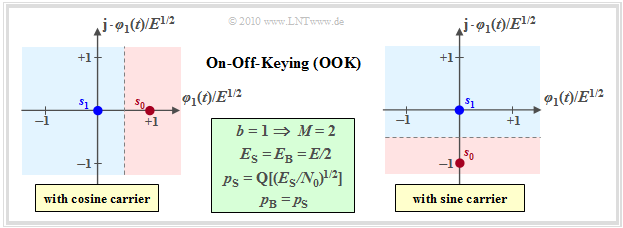
- $\rm OOK$ is a binary and one-dimensional modulation method, for example with $s_{1} \equiv 0$ and
- $\boldsymbol{s}_{0} = \{s_0,\ 0\}$ $($for cosinusoidal carrier, left graph$)$ resp.
- $\boldsymbol{s}_{0} = \{0,\ -s_0\}$ $($for sinusoidal carrier, right graph$)$.
- With coherent demodulation, the signal space constellation of the received signal is equal to that of the transmitted signal and again consists of the two points $\boldsymbol{r}_0=\boldsymbol{s}_0$ and $\boldsymbol{r}_1=\boldsymbol{s}_1$.
- In this case, the AWGN noise is one-dimensional with variance $\sigma_{\rm AWGN}^2$ and one obtains corresponding to the "theory section" for the "symbol error probability":
- $$p_{\rm S} = {\rm Pr}(\boldsymbol{r}\ne \boldsymbol{s})= {\rm Q} \left ( \frac{s_0/2}{\sigma_{\rm AWGN}}\right ) = {\rm Q} \left ( \sqrt{ {E_{\rm S}}/{N_0}}\right ) \hspace{0.05cm}. $$
To this it should be noted:
- The function ${\rm Q}(x)$ is called the "Complementary Gaussian Error Function".
- The above equation applies to equally probable symbols with the decision threshold $G$ midway between $\boldsymbol{r}_0$ and $\boldsymbol{r}_1$.
- The distance of the two signal points from the decision threshold $G$ is thus respectively $\Delta G = s_0/2$ $($counter in the argument of the first $\rm Q$–function$)$.
- $E_{\rm S}=s_0^2/2 \cdot T$ denotes for this case the "average energy per symbol" and $N_0=2T \cdot \sigma_{\rm AWGN}^2$ is the $($one-sided$)$ AWGN noise power density.
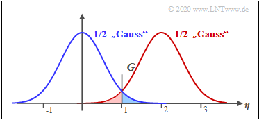
$\text{Example 1:}$ Let be $\sigma_{\rm AWGN}= 0.8$ and $s_{0} = 2$, ⇒ $G=1$ $($these values are normalized to $1\hspace{0.05cm} {\rm V})$.
The graph shows two "half Gaussian functions" around $s_1=0$ $($blue curve$)$ and $s_0=2$ $($red curve$)$. The threshold value $G$. The shaded areas mark the symbol error probability.
- According to the first equation, with $\Delta G = s_{0} -G= G-s_1 = 1$:
- $$p_{\rm S} = {\rm Q} ( 1/0.8 )= {\rm Q} ( 1.25 )\approx 10.56 \%.$$
- Similarly, the second equation provides: $E_{\rm S}/{N_0} = 1/4 \cdot s_0^2/\sigma_{\rm AWGN}^2 = 1.5615$:
- $$p_{\rm S} = {\rm Q} (\sqrt{1.5615} )\approx 10.56 \%.$$
Due to symmetry, the threshold $G=1$ is optimal. In this case, the red and blue shaded areas are equal ⇒ the symbols $\boldsymbol{s}_{0}$ and $\boldsymbol{s}_{1}$ are falsified in the same way.
With $G\ne 1$ there is a larger falsification probability. For example, with $G=0.6$:
- $$p_{\rm S} = {\rm Pr}(\boldsymbol{r}\ne \boldsymbol{s}) = {\rm Pr}(\boldsymbol{r_0} \cap \boldsymbol{s_1}) + {\rm Pr}(\boldsymbol{r_1} \cap \boldsymbol{s_0})= 1/2 \cdot {\rm Q} ( 0.75)+ 1/2 \cdot {\rm Q} ( 1.75)\approx 13.33\% .$$
Here the falsification probability for the symbol $\boldsymbol{s}_{1}$ ⇒ blue filled area ${\rm Pr}(\boldsymbol{r_0} \cap \boldsymbol{s_1}) \approx 11. 33\%$ is much larger than that of the symbol $\boldsymbol{s}_{0}$ ⇒ red filled area ${\rm Pr}(\boldsymbol{r_1} \cap \boldsymbol{s_0}) \approx 2\%$.
On–Off–Keying with noncoherent demodulation
The following diagram shows the structure $($in the equivalent low-pass range$)$ of the optimal OOK receiver for incoherent demodulation. See "Detailed description". According to this graph applies:
- The input signal $\boldsymbol{r}(t) = \boldsymbol{s}(t) \cdot {\rm e}^{\hspace{0.02cm}{\rm j}\hspace{0.03cm}\phi} + \boldsymbol{n}(t)$ at the receiver is generally complex because of the current phase angle $\phi$ and because of the complex noise term $\boldsymbol{n}(t)$.
- Now the correlation between the complex received signal $\boldsymbol{r}(t)$ and a "complex basis function" $\boldsymbol{\xi}(t)$ is required.
- The result is the $($complex$)$ detected value $\boldsymbol{r}$, from which the magnitude $y = |\boldsymbol{r}(t)|$ is formed as a real decision input.
- If $y \gt G$, then the estimated value $m_0$ for the symbol $\boldsymbol{s}_{0}$ is output, otherwise the estimated value $m_1$ for the symbol $\boldsymbol{s}_{1}$.
- Once again, the mean symbol error probability can be represented as the sum of two joint probabilities:
- $$p_{\rm S} = {\rm Pr}(\boldsymbol{r}\ne \boldsymbol{s}) = {\rm Pr}(\boldsymbol{r_0} \cap \boldsymbol{s_1}) + {\rm Pr}(\boldsymbol{r_1} \cap \boldsymbol{s_0}).$$
Error probability calculation considering Rayleigh and Rice distribution
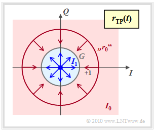
To calculate the symbol error probability for incoherent demodulation, we start from the following graph. Shown is the received signal in the equivalent low-pass region in the complex plane.
- The point $\boldsymbol{s_1}=0$ leads in the received signal again to $\boldsymbol{r_1}=0$.
- In contrast, $\boldsymbol{r}_0 = \boldsymbol{s}_0 \cdot {\rm e}^{\hspace{0.02cm}{\rm j}\hspace{0.03cm}\phi}$ can lie on any point of a circle with radius $1$ since the phase $\phi$ is unknown.
- The decision process taking into account that the AWGN noise is now to be interpreted in two dimensions, as indicated by the arrows in the graph.
- The decision region $I_1$ for symbol $\boldsymbol{s_1}$ is the blue filled circle with radius $G$, where the correct value of $G$ remains to be determined.
- If the received value $\boldsymbol{r}$ is outside this circle, i.e. in the red highlighted area $I_0$, the decision is in favor of $\boldsymbol{s_0}$.
$\rm Rayleigh\ portion$
Considering the AWGN–noise, $\boldsymbol{r_1}=\boldsymbol{s_1} + \boldsymbol{n_1}$. The noise component $\boldsymbol{n_1}$ has a "Rayleigh distribution" $($amount of the two mean-free Gaussian components for $I$ and $Q)$.
- Their conditional PDF is with the rotationally symmetric noise component $\eta$ with $\sigma=\sigma_{\rm AWGN}$ :
- $$f_{y\hspace{0.05cm}\vert \hspace{0.05cm}\boldsymbol{s_1}} (\eta \hspace{0.05cm}\vert \hspace{0.05cm} \boldsymbol{s_1})=\frac{\eta}{\sigma^2}\cdot {\rm e}^{-\eta^2 / ( 2 \hspace{0.05cm}\cdot \hspace{0.05cm}\sigma^2) } = f_{\rm Rayleigh}(\eta) .$$
- Thus one obtains for the conditional probability
- $${\rm Pr}(\boldsymbol{r_0}|\boldsymbol{s_1}) = \int_{G}^{\infty}f_{\rm Rayleigh}(\eta) \,{\rm d} \eta \hspace{0.05cm},$$
- and with the factor $1/2$ because of the equally probable transmitted symbols, the joint probability:
- $${\rm Pr}(\boldsymbol{r_0} \cap \boldsymbol{s_1}) = 1/2 \cdot {\rm Pr}(\boldsymbol{r_0}|\boldsymbol{s_1})= 1/2 \cdot \int_{G}^{\infty}f_{\rm Rayleigh}(\eta) \,{\rm d} \eta \hspace{0.05cm}.$$
$\rm Rice\ portion$
The noise component $\boldsymbol{n_0}$ has a "Rice distribution"
$($magnitude of Gaussian components with mean values $m_x$ and $m_y)$ ⇒ constant $C=\sqrt{m_x^2 + m_y^2}$
$($Note: In the applet, the constant $C$ is denoted by $C_{\rm Rice}$ $)$.
- $$f_{y\hspace{0.05cm}\vert \hspace{0.05cm}\boldsymbol{s_0}} (\eta \hspace{0.05cm}\vert \hspace{0.05cm} \boldsymbol{s_0})=\frac{\eta}{\sigma^2}\cdot{\rm e}^{-({C^2+\it \eta^{\rm 2} })/ ({\rm 2 \it \sigma^{\rm 2} })}\cdot {\rm I_0}(\frac{\it \eta\cdot C}{\sigma^{\rm 2} }) = f_{\rm Rice}(\eta) \hspace{1.4cm}{\rm with} \hspace{1.4cm} {\rm I_0}(\eta) = \sum_{k=0}^{\infty}\frac{(\eta/2)^{2k} }{k! \cdot {\rm \Gamma ({\it k}+1)} }.$$
This gives the second joint probability:
- $${\rm Pr}(\boldsymbol{r_1} \cap \boldsymbol{s_0}) = 1/2 \cdot \int_{0}^{G}f_{\rm Rice}(\eta) \,{\rm d} \eta \hspace{0.05cm}.$$
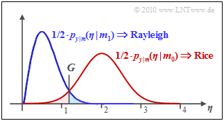
$\text{Example 2:}$ The graph shows the result of this equation for $\sigma_{\rm AWGN} = 0.5$ and $C_{\rm Rice} = 2$. The decision threshold is at $G \approx 1.25$. One can see from this plot:
- The symbol error probability $p_{\rm S}$ is the sum of the two colored areas. As in Example 1 for the coherent case:
- $$p_{\rm S} = {\rm Pr}(\boldsymbol{r}\ne \boldsymbol{s}) = {\rm Pr}(\boldsymbol{r_0} \cap \boldsymbol{s_1}) + {\rm Pr}(\boldsymbol{r_1} \cap \boldsymbol{s_0}).$$
- The area marked in blue gives the joint probability ${\rm Pr}(\boldsymbol{r_0} \cap \boldsymbol{s_1}) \approx 2.2\%$ This is calculated as the integral over half the Rayleigh PDF in the range from $G$ to $\infty$.
- The red highlighted area gives the joint probability ${\rm Pr}(\boldsymbol{r_1} \cap \boldsymbol{s_0}) \approx 2.4\%$ This is calculated as the integral over half the Rice PDF in the range from $0$ to $G$.
- Thus obtaining $p_{\rm S} \approx 4.6\%$. Note that the red and blue areas are not equal and that the optimal decision boundary $G_{\rm opt}$ is obtained from the intersection of the two curves.
- The optimal decision threshold $G_{\rm opt}$ is obtained as the intersection of the blue and red curves.
Exercises
- Select the number $(1,\ 2$, ... $)$ of the task to be processed. The number "0" corresponds to a "Reset": Setting as at the program start.
- A task description is displayed. Parameter values are adjusted. Solution after pressing "Sample solution".
- Always interpret the graphics and the numerical results. The symbols $s_0$ (adjustable) and ${s}_{1}\equiv 0$ are equal probability.
- For space reasons, in some of the following questions and sample solutions we also use $\sigma = \sigma_{\rm AWGN}$ and $C = C_{\rm Rice}$.
(1) We consider $\text{coherent}$ demodulation with $\sigma_{\rm AWGN} = 0.5$ and $s_0 = 2$. What is the smallest possible value for the symbol error probability $p_{\rm S}$?
- For coherent demodulation, the PDF of the reception signal is composed of two "half" Gaussian functions around $s_0 = 2$ $($red$)$ and $s_1 = 0$ $($blue$)$.
- Here the minimum $p_{\rm S}$ value results with $G=1$ and $\Delta G = s_{0} -G= G-s_1 = 1$ to $p_{\rm S}= {\rm Q} ( \Delta G/\sigma )={\rm Q} ( 1/0.5 )= {\rm Q} ( 2 )\approx 2.28 \%.$
- With $G=1$ both symbols are falsified equally. The blue area ${\rm Pr}(\boldsymbol{r_0} \cap \boldsymbol{s_1})$ is equal to the red area ${\rm Pr}(\boldsymbol{r_1} \cap \boldsymbol{s_0})$. Their sum gives $p_{\rm S}$.
- With $G=0.5$ the red area is almost zero. Nevertheless $p_{\rm S}\approx 8\%$ (sum of both areas) is more than twice as large as with $G_{\rm opt}=1$.
(2) Now let $\sigma = 0.75$. With what $s_0$ value does optimal $G$ give the same symbol error probability as in $(1)$? Then what is the quotient $E_{\rm S}/N_0$?
- In general $p_{\rm S}= {\rm Q}\big ( (s_0/2) / \sigma \big )$. If one increases $\sigma$ from $0. 5$ to $0.75$, then $s_0$ must also be increased ⇒ $s_0 = 3$ ⇒ $p_{\rm S}= {\rm Q} ( 1.5/ 0.75 )= {\rm Q} ( 2 )$.
- Except $p_{\rm S}= {\rm Q}\big ( (s_0/2) / \sigma \big )$ but also holds: $p_{\rm S}= {\rm Q} ( \sqrt{E_{\rm S}/N_0} )$. It follows: $p_{\rm S}= {\rm Q}(2) ={\rm Q} ( \sqrt{E_{\rm S}/N_0})$ ⇒ $\sqrt{E_{\rm S}/N_0}= 2$ ⇒ $E_{\rm S}/N_0= 4$.
- For control: $E_{\rm S}=s_0^2/2 \cdot T, \ N_0=2T \cdot \sigma^2$ ⇒ $E_{\rm S}/N_0 =s_0^2/(4 \cdot \sigma^2)= 3^2/(4 \cdot 0. 75^2)=4$. The same $E_{\rm S}/N_0 =4$ results for the problem $(1)$.
(3) Now consider $\text{non–coherent}$ demodulation with $\sigma_{\rm AWGN} = 0.75$, $C_{\rm Rice} = 2.25$ and $G=2$. What is the symbol error probability $p_{\rm S}$?
- For non–coherent demodulation, the PDF of the reception signal is composed of "half" a Rayleigh function $($blue$)$ and "half" a Rice function $($red$)$.
- ${\rm Pr}(\boldsymbol{r_0} \cap \boldsymbol{s_1}) \approx 1.43\%$ gives the proportions of the blue curve above $G =2$, and ${\rm Pr}(\boldsymbol{r_1} \cap \boldsymbol{s_0}) \approx 15. 18\%$ the proportions of the red curve below $G =2$.
- With $G=2$ the sum for the symbol error probability is $p_{\rm S}\approx 16.61\%$ , and with $G_{\rm opt}=1.58$ a slightly better value: $p_{\rm S}\approx 12.25\%$.
(4) Let $X$ be a Rayleigh random variable in general and $Y$ be a Rice random variable, each with above parameters. How large are ${\rm Pr}(X\le 2)$ and ${\rm Pr}(Y\le 2)$ ?
- It holds ${\rm Pr}(Y\le 2) = 2 \cdot {\rm Pr}(\boldsymbol{r_1} \cap \boldsymbol{s_0}) \approx 30.36\%$, since in the applet the Rice PDF is represented by the factor $1/2$.
- In the same way ${\rm Pr}(X> 2) = 2 \cdot {\rm Pr}(\boldsymbol{r_0} \cap \boldsymbol{s_1}) \approx 2.86\%$ ⇒ ${\rm Pr}(X \le 2)= 1-0.0286 = 97.14\%$.
(5) We consider the values $\sigma_{\rm AWGN} = 0.75$, $C_{\rm Rice} = 2.25$ and $G=G_{\rm opt}=1. 58$. How does $p_{\rm S}$ change when "Rice" is replaced by "Gauss" as best as possible?
- After the exact calculation, using the optimal threshold $G_{\rm opt}=1.58$: ${\rm Pr}(\boldsymbol{r_0} \cap \boldsymbol{s_1}) \approx 5. 44\%$, ${\rm Pr}(\boldsymbol{r_1} \cap \boldsymbol{s_0}) \approx 6.81\%$ ⇒ $p_{\rm S}\approx 12.25\%$.
- With the Gaussian approximation, for the same $G$ the first term is not changed. The second term increases to ${\rm Pr}(\boldsymbol{r_1} \cap \boldsymbol{s_0}) \approx 9.29\%$ ⇒ $p_{\rm S}\approx 14.73\%$.
- The new optimization of the threshold $G$ considering the Gaussian approximation leads to $G_{\rm opt}=1.53$ and $p_{\rm S}\approx 14.67\%$.
- The parameters of the Gaussian distribution are set as follows: mean $m_{\rm Gaussian}= C_{\rm Rice}=2.25$, standard deviation $\sigma_{\rm Gaussian}= \sigma_{\rm AWGN}=0.75$.
(6) How do the results change from $(5)$ with $\sigma_{\rm AWGN} = 0. 5$, $C_{\rm Rice} = 1.5$ and with $\sigma_{\rm AWGN} = 1$, $C_{\rm Rice} = 3$ respectively, each with $G=G_{\rm opt}$?
- With the optimal decision threshold $G_{\rm opt}$, the probabilities are the same, both for the exact Rice distribution and with the Gaussian approximation.
- For all three parameter sets, $E_{\rm S}/N_0= 2.25$. This suggests: The results with non–coherent demodulation depend on this characteristic value alone.
(7) Let the setting continue to be $\text{non–coherent/approximation}$ with $C_{\rm Rice} = 3$, $G=G_{\rm opt}$. Vary the AWGN standard deviation in the range $0.5 \le \sigma \le 1$.
Interpret the relative error ⇒ $\rm (False - Correct)/Correct$ as a function of the quotient $E_{\rm S}/N_0$.
- With $\sigma =0.5$ ⇒ $E_{\rm S}/N_0 = 9$ one obtains $p_{\rm S}^{\ \rm (exact)}\approx 0. 32\%$ and $p_{\rm S}^{\ \rm (approximate)}\approx 0.38\%$. The absolute error is $0.06\%$ and the relative error $18.75\%$.
- With $\sigma =1$ ⇒ $E_{\rm S}/N_0 = 2.25$ one obtains $p_{\rm S}^{\ \rm (exact)}\approx 12. 25\%$ and $p_{\rm S}^{\ \rm (approximate)}\approx 14.67\%$. The absolute error is $2.42\%$ and the relative error $19.75\%$.
- ⇒ The Gaussian approximation becomes better with larger $E_{\rm S}/N_0$. This statement can be seen more clearly from the absolute than from the relative error.
(8) Now repeat the last experiment with $\text{coherent}$ demodulation and $s_0 = 3$, $G=G_{\rm opt}$. What conclusion does the comparison with $(7)$ allow?
- The comparison of $(7)$ and $(8)$ shows: For each $E_{\rm S}/N_0$ there is a greater (worse) symbol error probability with non–coherent demodulation.
- For $E_{\rm S}/N_0= 9$: $p_{\rm S}^{\ \rm (coherent)}\approx 0.13\%$ and $p_{\rm S}^{\ \rm (non–coherent)}\approx 0.32\%$. And for $E_{\rm S}/N_0= 2.25$: $p_{\rm S}^{\ \rm (coherent)}\approx 6.68\%$ and $p_{\rm S}^{\ \rm (non–coherent)}\approx 12.25\%$.
- The simpler realization of the incoherent demodulator (no clock synchronization) causes a loss of quality ⇒ greater error probability.
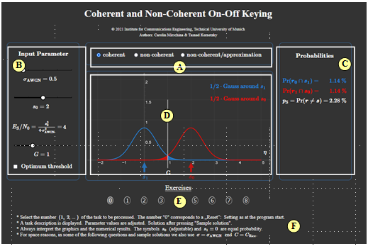
Applet Manual
(A) Selection:
- coherent,
- Incoherent,
- Incoherent with approximation.
(B) Parameter input:
- $\sigma_{\rm AWGN}$,
- $s_0$,
- $E_{\rm S}/N_0$,
- $G_{\rm opt}$
(C) Numerical output area of probabilities.
(D) Graphical output area of PDF proportions.
(E) Exercise selection
(F) Questions and solutions
About the Authors
This interactive calculation tool was designed and implemented at the Institute for Communications Engineering at the Technical University of Munich.
- The first version was created in 2011 by Martin Völkl as part of his diploma thesis with “FlashMX – Actionscript” (Supervisor: Günter Söder and Klaus Eichin).
- In 2020 the program was redesigned via HTML5/JavaScript by Carolin Mirschina in the context of a working student activity (Supervisor: Tasnád Kernetzky ).
- Last revision and English version 2021 by Carolin Mirschina.
- The conversion of this applet was financially supported by "Studienzuschüsse" (TUM Department of Electrical and Computer Engineering). We thank.
