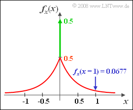
*The exercise belongs to the chapter [[Theory_of_Stochastic_Signals/Cumulative_Distribution_Function|cumulative distribution function]].
*The exercise belongs to the chapter [[Theory_of_Stochastic_Signals/Cumulative_Distribution_Function|Cumulative Distribution Function]].
*Reference is made to the chapter [[Theory_of_Stochastic_Signals/Probability_Density_Function]].
*Reference is made to the chapter [[Theory_of_Stochastic_Signals/Probability_Density_Function|Probability Density Function]].
*The topic of this chapter is illustrated with examples in the (German language) learning video [[Zusammenhang_zwischen_WDF_und_VTF_(Lernvideo)|Zusammenhang zwischen WDF und VTF]] $\Rightarrow$ relationship between PDF and CDF.
*The topic of this chapter is illustrated with examples in the (German language) learning video <br> [[Zusammenhang_zwischen_WDF_und_VTF_(Lernvideo)|"Zusammenhang zwischen WDF und VTF"]] $\Rightarrow$ "Relationship between PDF and CDF".
Line 27:
Line 27:
<quiz display=simple>
<quiz display=simple>
{What properties of a CDF hold when the random variable has no limits?
{What properties of the CDF hold when the random variable has no limits?
|type="[]"}
|type="[]"}
+ The CDF increases from $0$ to $1$ at least weakly monotonically.
+ The CDF increases from $0$ to $1$ at least weakly monotonically.
- The $F_x(r)$–values $0$ and $1$ are possible für finite $r$–values.
- The $F_x(r)$ values $0$ and $1$ are possible for finite $r$ values.
+A horizontal section indicates that in this range the random size has no proportions.
+A horizontal section indicates that in this range the random size has no proportions.
+Vertical sections are possible.
+Vertical sections are possible.
Line 64:
Line 64:
===Solution===
===Solution===
{{ML-Kopf}}
{{ML-Kopf}}
'''(1)''' The <u>statements 1, 3 and 4</u> are always correct:
'''(1)''' The <u>statements 1, 3 and 4</u> are always correct:
*A horizontal intercept in the VTF indicates that the random size has no values in that region.
*A horizontal intercept in the CDF indicates that the random variable has no values in that region.
*In contrast, a vertical intercept in the VTF indicates a Dirac function in the WDF $($at the same location $x_0)$ .
*In contrast, a vertical intercept in the CDF indicates a Dirac delta function in the PDF $($at the same location $x_0)$.
*This means that the random size takes the value $x_0$ very frequently, namely with finite probability.
*This means that the random variable takes the value $x_0$ very frequently, namely with finite probability.
*All other values occur exactly with probability $0$ .
*All other values occur exactly with probability $0$.
*If, however $x$ is limited to the range from $x_{\rm min}$ to $x_{\rm max}$ then $F_x(r) = 0$ für $r < x_{\rm min}$ and $F_x(r) = 1$ für $r > x_{\rm max}$.
*If, however $x$ is limited to the range from $x_{\rm min}$ to $x_{\rm max}$ then $F_x(r) = 0$ for $r < x_{\rm min}$ and $F_x(r) = 1$ for $r > x_{\rm max}$.
*In this special case, the second statement would also be true.
*In this special case, the second statement would also be true.
'''(2)''' The sought probability can be calculated from the difference of the VTF–values at the boundaries:
'''(2)''' The sought probability can be calculated from the difference of the CDF values at the boundaries:
The topic of this chapter is illustrated with examples in the (German language) learning video "Zusammenhang zwischen WDF und VTF" $\Rightarrow$ "Relationship between PDF and CDF".
A horizontal intercept in the CDF indicates that the random variable has no values in that region.
In contrast, a vertical intercept in the CDF indicates a Dirac delta function in the PDF $($at the same location $x_0)$.
This means that the random variable takes the value $x_0$ very frequently, namely with finite probability.
All other values occur exactly with probability $0$.
If, however $x$ is limited to the range from $x_{\rm min}$ to $x_{\rm max}$ then $F_x(r) = 0$ for $r < x_{\rm min}$ and $F_x(r) = 1$ for $r > x_{\rm max}$.
In this special case, the second statement would also be true.
(2) The sought probability can be calculated from the difference of the CDF values at the boundaries: