A spread spectrum system is considered according to the given diagram in the equivalent low-pass range:
A spread spectrum system is considered according to the given diagram in the equivalent low-pass range:
*Let the digital signal $q(t)$ possess the power density spectrum ${\it \Phi}_q(f)$, which is to be approximated as rectangular with bandwidth $B = 1/T = 100\ \rm kHz$ (a rather unrealistic assumption):
*Let the digital signal $q(t)$ possess the power-spectral density ${\it \Phi}_q(f)$, which is to be approximated as rectangular with bandwidth $B = 1/T = 100\ \rm kHz$ (a rather unrealistic assumption):
*Thus, in the low-pass range, the bandwidth (only the components at positive frequencies) is equal to $B/2$ and the bandwidth in the band-pass range is $B$.
*Thus, in the low-pass range, the bandwidth (only the components at positive frequencies) is equal to $B/2$ and the bandwidth in the band-pass range is $B$.
*The band spreading is done by multiplication with the PN sequence $c(t)$ of the chip duration $T_c = T/100$ <br>("PN" stands for "pseudo-noise").
*The band spreading is done by multiplication with the PN sequence $c(t)$ of the chip duration $T_c = T/100$ <br>("PN" stands for "pseudo-noise").
*To simplify matters, the following applies to the autocorrelation function:
*To simplify matters, the following applies to the auto-correlation function:
*At the receiver, the same spreading sequence $c(t)$ is again added phase-synchronously.
*At the receiver, the same spreading sequence $c(t)$ is again added phase-synchronously.
Line 35:
Line 28:
<quiz display=simple>
<quiz display=simple>
{What is the power density spectrum ${\it \Phi}_c(f )$ of the spreading signal $c(t)$? What value results at the frequency $f = 0$?
{What is the power-spectral density ${\it \Phi}_c(f )$ of the spreading signal $c(t)$? What value results at the frequency $f = 0$?
'''(1)''' The power density spectrum ${\it \Phi}_c(f)$ is the Fourier transform of the triangular AKF, which can be represented with rectangles of width $T_c$ as follows:
'''(1)''' The power-spectral density $\rm (PDS)$ ${\it \Phi}_c(f)$ is the Fourier transform of the triangular ACF, which can be represented with rectangles of width $T_c$ as follows:
*that $B_c$ is given by the first zero of the $\rm si^2$ function in the equivalent low-pass range,
*that $B_c$ is given by the first zero of the $\rm sinc^2$ function in the equivalent low-pass range,
*but at the same time also gives the equivalent (equal area) bandwidth in the bandpass region.
*but at the same time also gives the equivalent (equal area) bandwidth in the band-pass region.
'''(3)''' <u>Solutions 2 and 5</u> are correct:
'''(3)''' <u>Solutions 2 and 5</u> are correct:
*The LDS ${\it \Phi}_s(f)$ results from the convolution of ${\it \Phi}_q(f)$ and ${\it \Phi}_c(f)$. This actually gives $B_s = B_c + B$ for the bandwidth of the transmitted signal.
*The PDS ${\it \Phi}_s(f)$ results from the convolution of ${\it \Phi}_q(f)$ and ${\it \Phi}_c(f)$. This actually gives $B_s = B_c + B$ for the bandwidth of the transmitted signal.
*Since the spreading signal $c(t) ∈ \{+1, –1\}$ multiplied by itself always gives the value $1$, naturally $b(t) ≡ q(t)$ and consequently $B_b = B$.
*Since the spreading signal $c(t) ∈ \{+1, –1\}$ multiplied by itself always gives the value $1$, naturally $b(t) ≡ q(t)$ and consequently $B_b = B$.
*Obviously, the bandwidth $B_b$ of the band compressed signal is not equal to $2B_c + B$, although the convolution ${\it \Phi}_s(f) ∗ {\it \Phi}_c(f)$ suggests this.
*Obviously, the bandwidth $B_b$ of the band compressed signal is not equal to $2B_c + B$, although the convolution ${\it \Phi}_s(f) ∗ {\it \Phi}_c(f)$ suggests this.
*This is due to the fact that the power density spectra must not be convolved, but the spectral functions (amplitude spectra) $S(f)$ and $C(f)$ must be assumed, taking into account the phase relations.
*This is due to the fact that the power density spectra must not be convolved, but the spectral functions (amplitude spectra) $S(f)$ and $C(f)$ must be assumed, taking into account the phase relations.
*Only then can the LDS $B(f)$ be determined from ${\it \Phi}_b(f)$. Clearly, the following is also true: $C(f) ∗ C(f) = δ(f)$.
*Only then can the PDS $B(f)$ be determined from ${\it \Phi}_b(f)$. Clearly, the following is also true: $C(f) ∗ C(f) = δ(f)$.
'''(4)''' Only the <u>first solution</u> is correct. The solution shall be clarified by the diagram at the end of the page:
'''(4)''' Only the <u>first solution</u> is correct. The solution shall be clarified by the diagram at the end of the page:
*In the upper diagram the LDS ${\it \Phi}_i(f)$ of the narrowband interferer is approximated by two Dirac functions at $±f_{\rm T}$ with weights $P_{\rm I}/2$. Also plotted is the bandwidth $B = 0.1 \ \rm MHz$ (not quite true to scale).
*In the upper diagram the PDS ${\it \Phi}_i(f)$ of the narrowband interferer is approximated by two Dirac delta functions at $±f_{\rm T}$ with weights $P_{\rm I}/2$. Also plotted is the bandwidth $B = 0.1 \ \rm MHz$ (not quite true to scale).
*The receiver-side multiplication with $c(t)$ – actually with the function of the band compression, at least with respect to the useful part of $r(t)$ – causes a band spreading with respect to the interference signal $i(t)$. Without considering the useful signal, $b(t) = n(t) = i(t) · c(t)$. It follows:
*The receiver-side multiplication with $c(t)$ – actually with the function of the band compression, at least with respect to the useful part of $r(t)$ – causes a band spreading with respect to the interference signal $i(t)$. Without considering the useful signal, $b(t) = n(t) = i(t) · c(t)$. It follows:
[[File:P_ID1870__Mod_A_5_2c.png|right|frame|Power density spectra before and after band spreading]]
[[File:P_ID1870__Mod_A_5_2c.png|right|frame|Power density spectra before and after band spreading]]
*Note that $n(t)$ is used here only as an abbreviation and does not denote AWGN noise.
*Note that $n(t)$ is used here only as an abbreviation and does not denote AWGN noise.
*In a narrow range around the carrier frequency $f_{\rm T} = 30 \ \rm MHz$, the LDS ${\it \Phi}_n(f)$ is almost constant. Thus, the interference power after band spreading is:
*In a narrow range around the carrier frequency $f_{\rm T} = 30 \ \rm MHz$, the PDS ${\it \Phi}_n(f)$ is almost constant. Thus, the interference power after band spreading is:
*This means: the interference power is reduced by the factor $J = T/T_c$ by band spreading, which is why $J$ is often called spreading gain.
*This means: The interference power is reduced by the factor $J = T/T_c$ by band spreading, which is why $J$ is often called "spreading gain".
*However, such a spreading gain is only given for a narrowband interferer.
*However, such a "spreading gain" is only given for a narrowband interferer.
A spread spectrum system is considered according to the given diagram in the equivalent low-pass range:
Let the digital signal $q(t)$ possess the power-spectral density ${\it \Phi}_q(f)$, which is to be approximated as rectangular with bandwidth $B = 1/T = 100\ \rm kHz$ (a rather unrealistic assumption):
Thus, in the low-pass range, the bandwidth (only the components at positive frequencies) is equal to $B/2$ and the bandwidth in the band-pass range is $B$.
The band spreading is done by multiplication with the PN sequence $c(t)$ of the chip duration $T_c = T/100$ ("PN" stands for "pseudo-noise").
To simplify matters, the following applies to the auto-correlation function:
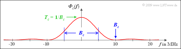
(1) The power-spectral density $\rm (PDS)$ ${\it \Phi}_c(f)$ is the Fourier transform of the triangular ACF, which can be represented with rectangles of width $T_c$ as follows:
that $B_c$ is given by the first zero of the $\rm sinc^2$ function in the equivalent low-pass range,
but at the same time also gives the equivalent (equal area) bandwidth in the band-pass region.
(3)Solutions 2 and 5 are correct:
The PDS ${\it \Phi}_s(f)$ results from the convolution of ${\it \Phi}_q(f)$ and ${\it \Phi}_c(f)$. This actually gives $B_s = B_c + B$ for the bandwidth of the transmitted signal.
Since the spreading signal $c(t) ∈ \{+1, –1\}$ multiplied by itself always gives the value $1$, naturally $b(t) ≡ q(t)$ and consequently $B_b = B$.
Obviously, the bandwidth $B_b$ of the band compressed signal is not equal to $2B_c + B$, although the convolution ${\it \Phi}_s(f) ∗ {\it \Phi}_c(f)$ suggests this.
This is due to the fact that the power density spectra must not be convolved, but the spectral functions (amplitude spectra) $S(f)$ and $C(f)$ must be assumed, taking into account the phase relations.
Only then can the PDS $B(f)$ be determined from ${\it \Phi}_b(f)$. Clearly, the following is also true: $C(f) ∗ C(f) = δ(f)$.
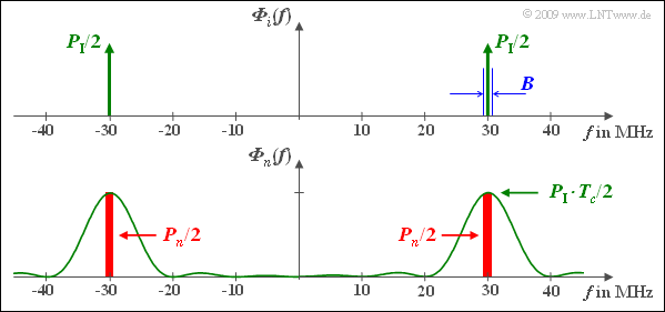
(4) Only the first solution is correct. The solution shall be clarified by the diagram at the end of the page:
In the upper diagram the PDS ${\it \Phi}_i(f)$ of the narrowband interferer is approximated by two Dirac delta functions at $±f_{\rm T}$ with weights $P_{\rm I}/2$. Also plotted is the bandwidth $B = 0.1 \ \rm MHz$ (not quite true to scale).
The receiver-side multiplication with $c(t)$ – actually with the function of the band compression, at least with respect to the useful part of $r(t)$ – causes a band spreading with respect to the interference signal $i(t)$. Without considering the useful signal, $b(t) = n(t) = i(t) · c(t)$. It follows:
Power density spectra before and after band spreading
Note that $n(t)$ is used here only as an abbreviation and does not denote AWGN noise.
In a narrow range around the carrier frequency $f_{\rm T} = 30 \ \rm MHz$, the PDS ${\it \Phi}_n(f)$ is almost constant. Thus, the interference power after band spreading is: