Wir betrachten zweidimensionales Rauschen $\boldsymbol{n} = (n_1, n_2)$.
We consider two-dimensional noise $\boldsymbol{n} = (n_1, n_2)$.
Die beiden Rauschvariablen sind „<i>independent and identically distributed</i> ”, abgekürzt i.i.d., und besitzen beide jeweils eine Laplace–Wahrscheinlichkeitsdichte:
The two noise variables are "independent and identically distributed", abbreviated "i.i.d.", and each has a Laplace probability density function $\rm (PDF)$:
:$$p_{n_1}(x) \hspace{-0.1cm} \ = \ \hspace{-0.1cm} K \cdot {\rm e}^{- a \hspace{0.03cm}\cdot \hspace{0.03cm} |x|} \hspace{0.05cm},$$
:$$p_{n_1}(x) \hspace{-0.1cm} \ = \ \hspace{-0.1cm} K \cdot {\rm e}^{- a \hspace{0.03cm}\cdot \hspace{0.03cm} |x|} \hspace{0.05cm},$$
:$$ p_{n_2}(y) \hspace{-0.1cm} \ = \ \hspace{-0.1cm} K \cdot {\rm e}^{- a \hspace{0.03cm}\cdot \hspace{0.03cm} |y|} \hspace{0.05cm}. $$
:$$ p_{n_2}(y) \hspace{-0.1cm} \ = \ \hspace{-0.1cm} K \cdot {\rm e}^{- a \hspace{0.03cm}\cdot \hspace{0.03cm} |y|} \hspace{0.05cm}. $$
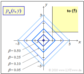
*Die 2D–Wahrscheinlichkeitsdichtefunktion $p_{\it \boldsymbol{n}}(x, y)$ ist in der Grafik dargestellt.
*The two-dimensional probability density function $p_{\it \boldsymbol{n}}(x, y)$ is shown in the graph.
*Zur Vereinfachung der Schreibweise werden hier die Realisierungen von $n_1$ und $n_2$ mit $x$ und $y$ bezeichnet.
*To simplify notation, the realizations of $n_1$ and $n_2$ are denoted here by $x$ and $y$, respectively.
''Hinweise:''
* Die Aufgabe gehört zum Kapitel [[Digitalsignal%C3%BCbertragung/Approximation_der_Fehlerwahrscheinlichkeit| Approximation der Fehlerwahrscheinlichkeit]].
Notes:
* The exercise belongs to the chapter [[Digital_Signal_Transmission/Approximation_of_the_Error_Probability|"Approximation of the Error Probability"]].
* Beachten Sie bitte, dass in Teilaufgabe '''(6)''' das sich ergebende Integral aufgrund der Betragsbildung in mehrere Teilintegrale aufgespalten werden muss.
* We would like to refer to the (German language) interactive SWF applet [[Applets:2D_Laplace|"2D Laplace"]].
* The integral resulting in subtask '''(6)''' must be split into several partial integrals due to the magnitude formation.
*Furthermore, it holds: $\int_{0}^{\infty} x^2 \cdot {\rm e}^{-a \hspace{0.03cm}\cdot \hspace{0.03cm} x} \,{\rm d} x = {2}/{a^3} \hspace{0.05cm}.$
===Fragebogen===
===Questions===
<quiz display=simple>
<quiz display=simple>
{Wie groß ist die Konstante $K$ der 1D–WDF?
{What is the size of the constant $K$ of the one-dimensional PDF?
|type="[]"}
|type="()"}
- $K = 1$.
- $K = 1$.
+ $K = a/2$
+ $K = a/2$
- $K = 1/a$.
- $K = 1/a$.
{Es sei $a = 1$. Wie groß sind der Mittelwert ${\rm E}\big[n_i \big]$ und die Varianz $\sigma^2 = {\rm E}\big[n_i^2\big]$ der beiden 1D–Zufallsgrößen? $(i = 1, 2)$
{Let $a = 1$. What are the mean ${\rm E}\big[n_i \big]$ and the variance $\sigma^2 = {\rm E}\big[n_i^2\big]$ of the two one-dimensional random variables? $(i = 1,\ 2)$.
|type="{}"}
|type="{}"}
${\rm E}\big[n_i\big] \ = \ $ { 0. }
${\rm E}\big[n_i\big] \ = \ $ { 0. }
${\rm E}\big[n_i^2\big] \ = \ ${ 2 3% }
${\rm E}\big[n_i^2\big] \ = \ ${ 2 3% }
{Welche Form haben die Höhenlinien der 2D–WDF im ersten Quadranten?
{What is the shape of the contour lines of the two-dimensional PDF in the first quadrant?
|type="[]"}
|type="()"}
+ Es sind Geraden.
+ They are straight lines.
- Es sind Hyperbeln.
- They are hyperbolas.
- Es sind Kreise.
- They are circles.
{Es sei weiterhin $a = 1$. Wie groß ist die Wahrscheinlichkeit, dass sowohl $n_1$ als auch $n_2$ negativ sind?
{Let further $a = 1$. What is the probability that both $n_1$ and $n_2$ are negative?
[[File:P_ID2045__Dig_Z_4_9c.png|right|frame|Höhenlinien der 2D-Laplaceverteilung]]
'''(3)''' Richtig ist der <u>Lösungsvorschlag 1</u>:
'''(3)''' <u>Solution 1</u> is correct:
*Im ersten Quadranten ($x ≥ 0, y ≥ 0$) kann auf die Betragsbildung verzichtet werden. Dann gilt für die 2D–WDF:
*In the first quadrant $(x ≥ 0, y ≥ 0)$, the magnitude formation can be omitted. Then the two-dimensional PDF is given by:
:$$\boldsymbol{ p }_{\boldsymbol{ n }} (x,\hspace{0.15cm} y) = {a^2}/{4} \cdot {\rm e}^{- a \hspace{0.03cm}\cdot \hspace{0.03cm}x} \cdot {\rm e}^{- a \hspace{0.03cm}\cdot \hspace{0.03cm}y }= {a^2}/{4} \cdot {\rm e}^{- a \hspace{0.03cm}\cdot \hspace{0.03cm}(x+y)}\hspace{0.05cm}.$$
:$$\boldsymbol{ p }_{\boldsymbol{ n }} (x,\hspace{0.15cm} y) = {a^2}/{4} \cdot {\rm e}^{- a \hspace{0.03cm}\cdot \hspace{0.03cm}x} \cdot {\rm e}^{- a \hspace{0.03cm}\cdot \hspace{0.03cm}y }= {a^2}/{4} \cdot {\rm e}^{- a \hspace{0.03cm}\cdot \hspace{0.03cm}(x+y)}\hspace{0.05cm}.$$
*Eine Höhenlinie mit dem Faktor $\beta$ gegenüber dem Maximum hat dann den folgenden Verlauf ($0 < \beta < 1$):
*A contour line with factor $\beta$ versus maximum then has the following shape $(0 < \beta < 1)$:
:$${\rm e}^{- a \hspace{0.03cm}\cdot \hspace{0.03cm}(x+y)} = \beta
:$${\rm e}^{- a \hspace{0.03cm}\cdot \hspace{0.03cm}(x+y)} = \beta\hspace{0.3cm} \Rightarrow \hspace{0.3cm} x + y = \frac{{\rm ln}\hspace{0.15cm}1/\beta}{a}\hspace{0.05cm}.$$
\hspace{0.3cm} \Rightarrow \hspace{0.3cm} x + y = \frac{{\rm ln}\hspace{0.15cm}1/\beta}{a}
\hspace{0.05cm}.$$
*Die Grafik zeigt die Höhenlinien für $a = 1$ und einige Werte von $\beta$, die jeweils ein um $45^\circ$ gedrehtes Quadrat ergeben ⇒ die Höhenlinien sind also Gerade..
*The graph shows the contour lines for $a = 1$ and some values of $\beta$, each giving a square rotated by $45^\circ$ ⇒ the contour lines are thus even.
* Wir weisen Sie auch auf das Interaktionsmodul [[Zweidimensionale Laplaceverteilung]] hin.
'''(4)''' Das hier betrachtete Wahrscheinlichkeitsereignis entspricht genau dem dritten Quadranten der oben skizzierten Verbund–WDF. Aufgrund der Symmetrie ist diese Wahrscheinlichkeit:
'''(4)''' The probability event considered here corresponds exactly to the third quadrant of the composite PDF sketched above.
Berücksichtigt ist die statistische Unabhängigkeit zwischen $n_1$ und $n_2$ sowie die Gleichheit $p_{\it n1}(x) = p_{\it n2}(y)$. Für $a = 1$ gilt:
*Considered is the statistical independence between $n_1$ and $n_2$ and the equality $p_{\it n1}(x) = p_{\it n2}(y)$. For $a = 1$ holds:
[[File:P_ID2046__Dig_Z_4_9f.png|right|frame|Aufteilung des Integrationsbereichs]]
[[File:P_ID2046__Dig_Z_4_9f.png|right|frame|Division of the integration domain]]
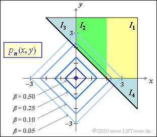
'''(6)''' Die hier betrachtete Region ist in der folgenden Grafik farbig markiert. Die Regionen erstrecken sich aber nach rechts und oben bis ins Unendliche. Die gesuchte Wahrscheinlichkeit ergibt sich zu
'''(6)''' The region considered here is highlighted in color in the following graph.
*However, the regions extend to the right and above to infinity.
Aufgrund der Betragsbildung ist eine Aufspaltung in Teilintegrale vorzunehmen. Nach oben und rechts erstrecken sich alle Gebiete bis ins Unendliche. Aufgrund der Symmetrie gilt $I_4 = I_3$.
*Because of the magnitude, a splitting into partial integrals has to be done.
:$$I_1 = {1}/{4} \cdot \int_{2}^{+\infty} \hspace{-0.15cm}{\rm e}^{-x} \int_{0}^{\infty}\hspace{-0.15cm}{\rm e}^{-y} \,{\rm d} y \,{\rm d} x =
{1}/{4} \cdot \int_{2}^{+\infty} {\rm e}^{-x} \,{\rm d} x ={1}/({4{\rm e}^2})\hspace{0.05cm},$$
*Upwards and to the right all areas extend to infinity.
:$$I_2 = {1}/{4} \cdot \hspace{-0.1cm} \int_{0}^{2} \hspace{-0.15cm}{\rm e}^{-x} \int_{2-x}^{\infty}\hspace{-0.15cm}{\rm e}^{-y} \,{\rm d} y \,{\rm d} x =
We consider two-dimensional noise $\boldsymbol{n} = (n_1, n_2)$.
The two noise variables are "independent and identically distributed", abbreviated "i.i.d.", and each has a Laplace probability density function $\rm (PDF)$:
$$p_{n_1}(x) \hspace{-0.1cm} \ = \ \hspace{-0.1cm} K \cdot {\rm e}^{- a \hspace{0.03cm}\cdot \hspace{0.03cm} |x|} \hspace{0.05cm},$$
$$ p_{n_2}(y) \hspace{-0.1cm} \ = \ \hspace{-0.1cm} K \cdot {\rm e}^{- a \hspace{0.03cm}\cdot \hspace{0.03cm} |y|} \hspace{0.05cm}. $$
The two-dimensional probability density function $p_{\it \boldsymbol{n}}(x, y)$ is shown in the graph.
To simplify notation, the realizations of $n_1$ and $n_2$ are denoted here by $x$ and $y$, respectively.
In the first quadrant $(x ≥ 0, y ≥ 0)$, the magnitude formation can be omitted. Then the two-dimensional PDF is given by:
$$\boldsymbol{ p }_{\boldsymbol{ n }} (x,\hspace{0.15cm} y) = {a^2}/{4} \cdot {\rm e}^{- a \hspace{0.03cm}\cdot \hspace{0.03cm}x} \cdot {\rm e}^{- a \hspace{0.03cm}\cdot \hspace{0.03cm}y }= {a^2}/{4} \cdot {\rm e}^{- a \hspace{0.03cm}\cdot \hspace{0.03cm}(x+y)}\hspace{0.05cm}.$$
A contour line with factor $\beta$ versus maximum then has the following shape $(0 < \beta < 1)$:
$${\rm e}^{- a \hspace{0.03cm}\cdot \hspace{0.03cm}(x+y)} = \beta\hspace{0.3cm} \Rightarrow \hspace{0.3cm} x + y = \frac{{\rm ln}\hspace{0.15cm}1/\beta}{a}\hspace{0.05cm}.$$
The graph shows the contour lines for $a = 1$ and some values of $\beta$, each giving a square rotated by $45^\circ$ ⇒ the contour lines are thus even.
(4) The probability event considered here corresponds exactly to the third quadrant of the composite PDF sketched above.