We consider two-dimensional noise $\boldsymbol{n} = (n_1, n_2)$.
We consider two-dimensional noise $\boldsymbol{n} = (n_1, n_2)$.
The two noise variables are "<i>independent and identically distributed</i> ", abbreviated i.i.d., and each has a Laplace probability density:
The two noise variables are "independent and identically distributed", abbreviated "i.i.d.", and each has a Laplace probability density function $\rm (PDF)$:
:$$p_{n_1}(x) \hspace{-0.1cm} \ = \ \hspace{-0.1cm} K \cdot {\rm e}^{- a \hspace{0.03cm}\cdot \hspace{0.03cm} |x|} \hspace{0.05cm},$$
:$$p_{n_1}(x) \hspace{-0.1cm} \ = \ \hspace{-0.1cm} K \cdot {\rm e}^{- a \hspace{0.03cm}\cdot \hspace{0.03cm} |x|} \hspace{0.05cm},$$
:$$ p_{n_2}(y) \hspace{-0.1cm} \ = \ \hspace{-0.1cm} K \cdot {\rm e}^{- a \hspace{0.03cm}\cdot \hspace{0.03cm} |y|} \hspace{0.05cm}. $$
:$$ p_{n_2}(y) \hspace{-0.1cm} \ = \ \hspace{-0.1cm} K \cdot {\rm e}^{- a \hspace{0.03cm}\cdot \hspace{0.03cm} |y|} \hspace{0.05cm}. $$
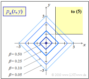
*The 2D probability density function $p_{\it \boldsymbol{n}}(x, y)$ is shown in the graph.
*The two-dimensional probability density function $p_{\it \boldsymbol{n}}(x, y)$ is shown in the graph.
*To simplify notation, the realizations of $n_1$ and $n_2$ are denoted here by $x$ and $y$, respectively.
*To simplify notation, the realizations of $n_1$ and $n_2$ are denoted here by $x$ and $y$, respectively.
''Notes:''
* The exercise belongs to the chapter [[Digital_Signal_Transmission/Approximation_of_the_Error_Probability|"Approximation of the Error Probability"]].
Notes:
* We would like to refer to the interactive applet [[Applets:2D_Laplace|"2D Laplace"]].
* The exercise belongs to the chapter [[Digital_Signal_Transmission/Approximation_of_the_Error_Probability|"Approximation of the Error Probability"]].
* The integral resulting in subtask '''(6)''' must be split into several partial integrals due to the magnitude formation.
*Furthermore, it holds:
* We would like to refer to the (German language) interactive SWF applet [[Applets:2D_Laplace|"2D Laplace"]].
* The integral resulting in subtask '''(6)''' must be split into several partial integrals due to the magnitude formation.
*Furthermore, it holds: $\int_{0}^{\infty} x^2 \cdot {\rm e}^{-a \hspace{0.03cm}\cdot \hspace{0.03cm} x} \,{\rm d} x = {2}/{a^3} \hspace{0.05cm}.$
Line 25:
Line 28:
===Questions===
===Questions===
<quiz display=simple>
<quiz display=simple>
{What is the size of the constant $K$ of the 1D PDF?
{What is the size of the constant $K$ of the one-dimensional PDF?
|type="[]"}
|type="()"}
- $K = 1$.
- $K = 1$.
+ $K = a/2$
+ $K = a/2$
- $K = 1/a$.
- $K = 1/a$.
{Let $a = 1$. What are the mean ${\rm E}\big[n_i \big]$ and variance $\sigma^2 = {\rm E}\big[n_i^2\big]$ of the two 1D random variables? $(i = 1, 2)$
{Let $a = 1$. What are the mean ${\rm E}\big[n_i \big]$ and the variance $\sigma^2 = {\rm E}\big[n_i^2\big]$ of the two one-dimensional random variables? $(i = 1,\ 2)$.
|type="{}"}
|type="{}"}
${\rm E}\big[n_i\big] \ = \ $ { 0. }
${\rm E}\big[n_i\big] \ = \ $ { 0. }
${\rm E}\big[n_i^2\big] \ = \ ${ 2 3% }
${\rm E}\big[n_i^2\big] \ = \ ${ 2 3% }
{What is the shape of the contour lines of the 2D PDF in the first quadrant?
{What is the shape of the contour lines of the two-dimensional PDF in the first quadrant?
|type="[]"}
|type="()"}
+ They are straight lines.
+ They are straight lines.
- They are hyperbolas.
- They are hyperbolas.
- They are circles.
- They are circles.
{Let further $a = 1$. What is the probability that both $n_1$ and $n_2$ are negative?
{Let further $a = 1$. What is the probability that both $n_1$ and $n_2$ are negative?
[[File:P_ID2045__Dig_Z_4_9c.png|right|frame|Contour lines of the 2D Laplace distribution]]
'''(3)''' <u>Solution 1</u> is correct:
'''(3)''' <u>Solution 1</u> is correct:
*In the first quadrant $(x ≥ 0, y ≥ 0)$, the magnitude formation can be omitted. Then the two-dimensional PDF is given by:
*In the first quadrant ($x ≥ 0, y ≥ 0$), the magnitude formation can be omitted. Then the 2D PDF is given by:
:$$\boldsymbol{ p }_{\boldsymbol{ n }} (x,\hspace{0.15cm} y) = {a^2}/{4} \cdot {\rm e}^{- a \hspace{0.03cm}\cdot \hspace{0.03cm}x} \cdot {\rm e}^{- a \hspace{0.03cm}\cdot \hspace{0.03cm}y }= {a^2}/{4} \cdot {\rm e}^{- a \hspace{0.03cm}\cdot \hspace{0.03cm}(x+y)}\hspace{0.05cm}.$$
:$$\boldsymbol{ p }_{\boldsymbol{ n }} (x,\hspace{0.15cm} y) = {a^2}/{4} \cdot {\rm e}^{- a \hspace{0.03cm}\cdot \hspace{0.03cm}x} \cdot {\rm e}^{- a \hspace{0.03cm}\cdot \hspace{0.03cm}y }= {a^2}/{4} \cdot {\rm e}^{- a \hspace{0.03cm}\cdot \hspace{0.03cm}(x+y)}\hspace{0.05cm}.$$
*A contour line with factor $\beta$ versus maximum then has the following shape ($0 < \beta < 1$):
*A contour line with factor $\beta$ versus maximum then has the following shape $(0 < \beta < 1)$:
:$${\rm e}^{- a \hspace{0.03cm}\cdot \hspace{0.03cm}(x+y)} = \beta
:$${\rm e}^{- a \hspace{0.03cm}\cdot \hspace{0.03cm}(x+y)} = \beta\hspace{0.3cm} \Rightarrow \hspace{0.3cm} x + y = \frac{{\rm ln}\hspace{0.15cm}1/\beta}{a}\hspace{0.05cm}.$$
\hspace{0.3cm} \Rightarrow \hspace{0.3cm} x + y = \frac{{\rm ln}\hspace{0.15cm}1/\beta}{a}
\hspace{0.05cm}.$$
*The graph shows the contour lines for $a = 1$ and some values of $\beta$, each giving a square rotated by $45^\circ$ ⇒ the contour lines are thus even.
*The graph shows the contour lines for $a = 1$ and some values of $\beta$, each giving a square rotated by $45^\circ$ ⇒ the contour lines are thus even.
'''(4)''' The probability event considered here corresponds exactly to the third quadrant of the composite PDF sketched above. Because of symmetry, this probability is:
'''(4)''' The probability event considered here corresponds exactly to the third quadrant of the composite PDF sketched above.
Considered is the statistical independence between $n_1$ and $n_2$ and the equality $p_{\it n1}(x) = p_{\it n2}(y)$. For $a = 1$ holds:
*Considered is the statistical independence between $n_1$ and $n_2$ and the equality $p_{\it n1}(x) = p_{\it n2}(y)$. For $a = 1$ holds:
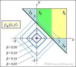
Because of the magnitude, a splitting into partial integrals has to be done. Upwards and to the right all areas extend to infinity. Because of the symmetry $I_4 = I_3$ is valid.
*Because of the magnitude, a splitting into partial integrals has to be done.
:$$I_1 = {1}/{4} \cdot \int_{2}^{+\infty} \hspace{-0.15cm}{\rm e}^{-x} \int_{0}^{\infty}\hspace{-0.15cm}{\rm e}^{-y} \,{\rm d} y \,{\rm d} x =
{1}/{4} \cdot \int_{2}^{+\infty} {\rm e}^{-x} \,{\rm d} x ={1}/({4{\rm e}^2})\hspace{0.05cm},$$
*Upwards and to the right all areas extend to infinity.
:$$I_2 = {1}/{4} \cdot \hspace{-0.1cm} \int_{0}^{2} \hspace{-0.15cm}{\rm e}^{-x} \int_{2-x}^{\infty}\hspace{-0.15cm}{\rm e}^{-y} \,{\rm d} y \,{\rm d} x =
We consider two-dimensional noise $\boldsymbol{n} = (n_1, n_2)$.
The two noise variables are "independent and identically distributed", abbreviated "i.i.d.", and each has a Laplace probability density function $\rm (PDF)$:
$$p_{n_1}(x) \hspace{-0.1cm} \ = \ \hspace{-0.1cm} K \cdot {\rm e}^{- a \hspace{0.03cm}\cdot \hspace{0.03cm} |x|} \hspace{0.05cm},$$
$$ p_{n_2}(y) \hspace{-0.1cm} \ = \ \hspace{-0.1cm} K \cdot {\rm e}^{- a \hspace{0.03cm}\cdot \hspace{0.03cm} |y|} \hspace{0.05cm}. $$
The two-dimensional probability density function $p_{\it \boldsymbol{n}}(x, y)$ is shown in the graph.
To simplify notation, the realizations of $n_1$ and $n_2$ are denoted here by $x$ and $y$, respectively.
In the first quadrant $(x ≥ 0, y ≥ 0)$, the magnitude formation can be omitted. Then the two-dimensional PDF is given by:
$$\boldsymbol{ p }_{\boldsymbol{ n }} (x,\hspace{0.15cm} y) = {a^2}/{4} \cdot {\rm e}^{- a \hspace{0.03cm}\cdot \hspace{0.03cm}x} \cdot {\rm e}^{- a \hspace{0.03cm}\cdot \hspace{0.03cm}y }= {a^2}/{4} \cdot {\rm e}^{- a \hspace{0.03cm}\cdot \hspace{0.03cm}(x+y)}\hspace{0.05cm}.$$
A contour line with factor $\beta$ versus maximum then has the following shape $(0 < \beta < 1)$:
$${\rm e}^{- a \hspace{0.03cm}\cdot \hspace{0.03cm}(x+y)} = \beta\hspace{0.3cm} \Rightarrow \hspace{0.3cm} x + y = \frac{{\rm ln}\hspace{0.15cm}1/\beta}{a}\hspace{0.05cm}.$$
The graph shows the contour lines for $a = 1$ and some values of $\beta$, each giving a square rotated by $45^\circ$ ⇒ the contour lines are thus even.
(4) The probability event considered here corresponds exactly to the third quadrant of the composite PDF sketched above.