Betrachtet wird ein ''Spread Spectrum System'' gemäß der vorliegenden Grafik im äquivalenten Tiefpassbereich:
of band spreading]]
*Das Digitalsignal $q(t)$ besitze das Leistungsdichtespektrum ${\it \Phi}_q(f)$, das als rechteckförmig mit der Bandbreite $B = 1/T = 100\ \rm kHz$ angenähert werden soll:
A spread spectrum system is considered according to the given diagram in the equivalent low-pass range:
:$${\it \Phi}_{q}(f) =
*Let the digital signal $q(t)$ possess the power-spectral density ${\it \Phi}_q(f)$, which is to be approximated as rectangular with bandwidth $B = 1/T = 100\ \rm kHz$ (a rather unrealistic assumption):
*Thus, in the low-pass range, the bandwidth (only the components at positive frequencies) is equal to $B/2$ and the bandwidth in the band-pass range is $B$.
\begin{array}{*{10}c} {\rm{f\ddot{u}r}}
*The band spreading is done by multiplication with the PN sequence $c(t)$ of the chip duration $T_c = T/100$ <br>("PN" stands for "pseudo-noise").
*At the receiver, the same spreading sequence $c(t)$ is again added phase-synchronously.
\end{array}$$
*The interference signal $i(t)$ is to be neglected for the time being.
*Im Tiefpassbereich ist somit die Bandbreite (nur die Anteile bei positiven Frequenzen) gleich $B/2$ und die Bandbreite im Bandpassbereich ist $B$.
*In subtask '''(4)''' $i(t)$ denotes a narrowband interferer at carrier frequency $f_{\rm T} = 30 \ \rm MHz = f_{\rm I}$ with power $P_{\rm I}$.
*Die Bandspreizung erfolgt durch Multiplikation mit der PN–Sequenz $c(t)$ der Chipdauer $T_c = T/100$ („PN” steht dabei für „Pseudo Noise”). Für die Autokorrelationsfunktion gelte vereinfachend:
*The influence of the (always present) AWGN noise $n(t)$ is not considered in this exercise.
*Beim Empfänger wird wieder die gleiche Spreizfolge $c(t)$ phasensynchron zugesetzt.
*Das Interferenzsignal $i(t)$ soll zunächst vernachlässigt werden. In der Teilaufgabe (4) bezeichnet $i(t)$ einen schmalbandigen Störer bei der Trägerfrequenz $f_{\rm T} = 30 \ \rm MHz = f_{\rm I}$ mit der Leistung $P_{\rm I}$.
*Der Einfluss des (stets vorhandenen) AWGN–Rauschens $n(t)$ wird in dieser Aufgabe nicht betrachtet.
''Hinweise:''
*Die Aufgabe gehört zum Kapitel [[Modulationsverfahren/PN–Modulation|PN–Modulation]].
*Sollte die Eingabe des Zahlenwertes „0” erforderlich sein, so geben Sie bitte „0.” ein.
===Fragebogen===
Note:
*This exercise belongs to the chapter [[Modulation_Methods/PN–Modulation|Direct-Sequence Spread Spectrum Modulation]].
===Questions===
<quiz display=simple>
<quiz display=simple>
{Wie lautet das Leistungsdichtespektrum ${\it \Phi}_c(f )$ des Spreizsignals $c(t)$? <br>Welcher Wert ergibt sich bei der Frequenz $f = 0$?
{What is the power-spectral density ${\it \Phi}_c(f )$ of the spreading signal $c(t)$? What value results at the frequency $f = 0$?
{Berechnen Sie die äquivalente Bandbreite $B_c$ des Spreizsignals als Breite des flächengleichen LDS–Rechtecks.
{Calculate the equivalent bandwidth $B_c$ of the spread signal as the width of the equal-area $\rm PDS$ rectangle.
|type="{}"}
|type="{}"}
$B_c \ = \ $ { 10 3% } $\ \rm MHz$
$B_c \ = \ $ { 10 3% } $\ \rm MHz$
{Welche Aussagen sind für die Bandbreiten der Signale $s(t)$ ⇒ $B_s$ und $b(t)$ ⇒ $B_b$ zutreffend? <br>Die (zweiseitige) Bandbreite von $q(t)$ ist $B$.
{Which statements are true for the bandwidths of the signals $s(t)$ ⇒ $B_s$ and $b(t)$ ⇒ $B_b$? The (two-sided) bandwidth of $q(t)$ is $B$.
|type="[]"}
|type="[]"}
- $B_s$ ist exakt gleich $B_c$.
- $B_s$ is exactly equal to $B_c$.
+ $B_s$ ist näherungsweise gleich $B_c + B$.
+ $B_s$ is approximately equal to $B_c + B$.
- $B_b$ ist exakt gleich $B_s$.
- $B_b$ is exactly equal to $B_s$.
- $B_b$ ist gleich $B_s + B_c = 2B_c + B$.
- $B_b$ is equal to $B_s + B_c = 2B_c + B$.
+ $B_b$ ist exakt gleich B.
+ $B_b$ is exactly equal to $B$.
{Welchen Einfluss hat eine Bandspreizung auf einen schmalbandigen Störer bei der Trägerfrequenz? Es gelte also $f_{\rm I} = f_{\rm T}$.
{What is the effect of band spreading on a "narrowband interferer" at the carrier frequency? Let $f_{\rm I} = f_{\rm T}$.
|type="[]"}
|type="[]"}
+ Der störende Einfluss wird durch Bandspreizung abgeschwächt.
+ The interfering influence is weakened by band spreading.
- Die Störleistung ist nur mehr halb so groß.
- The interfering power is only half as large.
- Die Störleistung wird durch die Bandspreizung nicht verändert.
- The interfering power is not changed by band spreading.
</quiz>
</quiz>
===Musterlösung===
===Solution===
{{ML-Kopf}}
{{ML-Kopf}}
'''1.''' Das Leistungsdichtesprektrum $Φ_c(f)$ ist die Fouriertransformierte der dreieckförmigen AKF, die mit Rechteckfunktionen der Breite $T_c$ wie folgt dargestellt werden kann:
'''(1)''' The power-spectral density $\rm (PDS)$ ${\it \Phi}_c(f)$ is the Fourier transform of the triangular ACF, which can be represented with rectangles of width $T_c$ as follows:
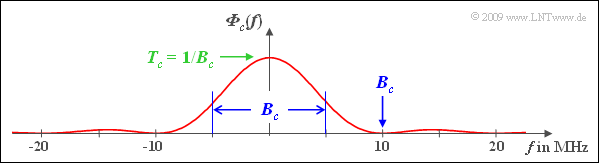
*that $B_c$ is given by the first zero of the $\rm sinc^2$ function in the equivalent low-pass range,
*but at the same time also gives the equivalent (equal area) bandwidth in the band-pass region.
'''(3)''' <u>Solutions 2 and 5</u> are correct:
*The PDS ${\it \Phi}_s(f)$ results from the convolution of ${\it \Phi}_q(f)$ and ${\it \Phi}_c(f)$. This actually gives $B_s = B_c + B$ for the bandwidth of the transmitted signal.
*Since the spreading signal $c(t) ∈ \{+1, –1\}$ multiplied by itself always gives the value $1$, naturally $b(t) ≡ q(t)$ and consequently $B_b = B$.
*Obviously, the bandwidth $B_b$ of the band compressed signal is not equal to $2B_c + B$, although the convolution ${\it \Phi}_s(f) ∗ {\it \Phi}_c(f)$ suggests this.
*This is due to the fact that the power density spectra must not be convolved, but the spectral functions (amplitude spectra) $S(f)$ and $C(f)$ must be assumed, taking into account the phase relations.
*Only then can the PDS $B(f)$ be determined from ${\it \Phi}_b(f)$. Clearly, the following is also true: $C(f) ∗ C(f) = δ(f)$.
'''2.''' Gemäß der vorgegebenen Definition gilt mit $T_c = T/100 = 0.1 μs$:
Die nachfolgende Grafik verdeutlicht, dass $B_c$ durch die erste Nullstelle der $si^2$–Funktion im äquivalenten Tiefpassbereich vorgegeben wird, aber auch gleichzeitig die äquivalente (flächengleiche) Bandbreite im Bandpassbereich angibt.
[[File:P_ID1869__Mod_A_5_2b.png|right|]]
'''3.''' Das LDS $Φ_s(f)$ ergibt sich aus der Faltung von $Φ_q(f)$ und $Φ_c(f)$. Damit ergibt sich für die Bandbreite des Sendesignals tatsächlich $B_s = B_c + B$. Da das Spreizsignal $c(t)$ ∈ {+1, –1} mit sich selbst multipliziert immer den Wert 1 ergibt, ist natürlich $b(t) ≡ q(t)$ und demzufolge $B_b = B$. Offensichtlich ist, dass die Bandbreite $B_b$ des bandgestauchten Signals ungleich $2B_c + B$ ist, obwohl die Faltung $Φ_s(f) ∗ Φ_c(f)$ dies suggeriert. Dies hängt damit zusammen, dass nicht die Leistungsdichtespektren gefaltet werden dürfen, sondern von den Spektralfunktionen (Amplitudenspektren) $S(f)$ und $C(f)$ unter Berücksichtigung der Phasenbeziehungen auszugehen ist. Erst danach kann aus $B(f)$ das LDS $Φ_b(f)$ bestimmt werden. Es gilt offensichtlich auch: $C(f) ∗ C(f) = δ(f)$. Richtig sind also die Lösungsvorschläge 2 und 5.
'''(4)''' Only the <u>first solution</u> is correct. The solution shall be clarified by the diagram at the end of the page:
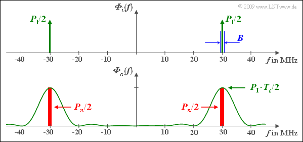
*In the upper diagram the PDS ${\it \Phi}_i(f)$ of the narrowband interferer is approximated by two Dirac delta functions at $±f_{\rm T}$ with weights $P_{\rm I}/2$. Also plotted is the bandwidth $B = 0.1 \ \rm MHz$ (not quite true to scale).
'''4.''' Die Lösung soll anhand einer Skizze verdeutlicht werden. Im oberen Diagramm ist das LDS $Φ_i(f)$ des Schmalbandstörers durch zwei Diracfunktionen bei $±f_T$ mit Gewichten $P_I/2$ angenähert. Eingezeichnet ist auch die Bandbreite $B = 0.1 MHz$ (nicht ganz maßstäblich).
*The receiver-side multiplication with $c(t)$ – actually with the function of the band compression, at least with respect to the useful part of $r(t)$ – causes a band spreading with respect to the interference signal $i(t)$. Without considering the useful signal, $b(t) = n(t) = i(t) · c(t)$. It follows:
[[File:P_ID1870__Mod_A_5_2c.png|right|frame|Power density spectra before and after band spreading]]
Die empfängerseitige Multiplikation mit $c(t)$ – eigentlich mit der Funktion der Bandstauchung, zumindest bezüglich des Nutzanteils von $r(t)$ – bewirkt hinsichtlich des Störsignals i(t) eine Bandspreizung. Ohne Berücksichtigung des Nutzsignals ist $b(t) = n(t) = i(t) · c(t)$. Daraus folgt:
*Note that $n(t)$ is used here only as an abbreviation and does not denote AWGN noise.
*In a narrow range around the carrier frequency $f_{\rm T} = 30 \ \rm MHz$, the PDS ${\it \Phi}_n(f)$ is almost constant. Thus, the interference power after band spreading is:
Anzumerken ist, dass $n(t)$ hier nur als Abkürzung verwendet wird und nicht wie sonst AWGN–Rauschen bezeichnet. In einem engen Bereich um die Trägerfrequenz $f_T = 30 MHz$ ist das LDS $Φ_n(f)$ nahezu konstant. Damit gilt für die Störleistung nach der Bandspreizung:
*This means: The interference power is reduced by the factor $J = T/T_c$ by band spreading, which is why $J$ is often called "spreading gain".
*However, such a "spreading gain" is only given for a narrowband interferer.
Das bedeutet: Die Störleistung wird durch Bandspreizung um den Faktor $J = T/T_c$ herabgesetzt, weshalb J häufig auch als Spreizgewinn bezeichnet wird. Ein solcher Spreizgewinn ist allerdings nur bei einem Schmalbandstörer gegeben.
Richtig ist somit der erste Lösungsvorschlag.
{{ML-Fuß}}
{{ML-Fuß}}
Line 85:
Line 95:
[[Category:Aufgaben zu Modulationsverfahren|^5.2 PN–Modulation^]]
A spread spectrum system is considered according to the given diagram in the equivalent low-pass range:
Let the digital signal $q(t)$ possess the power-spectral density ${\it \Phi}_q(f)$, which is to be approximated as rectangular with bandwidth $B = 1/T = 100\ \rm kHz$ (a rather unrealistic assumption):
Thus, in the low-pass range, the bandwidth (only the components at positive frequencies) is equal to $B/2$ and the bandwidth in the band-pass range is $B$.
The band spreading is done by multiplication with the PN sequence $c(t)$ of the chip duration $T_c = T/100$ ("PN" stands for "pseudo-noise").
To simplify matters, the following applies to the auto-correlation function:
(1) The power-spectral density $\rm (PDS)$ ${\it \Phi}_c(f)$ is the Fourier transform of the triangular ACF, which can be represented with rectangles of width $T_c$ as follows:
that $B_c$ is given by the first zero of the $\rm sinc^2$ function in the equivalent low-pass range,
but at the same time also gives the equivalent (equal area) bandwidth in the band-pass region.
(3)Solutions 2 and 5 are correct:
The PDS ${\it \Phi}_s(f)$ results from the convolution of ${\it \Phi}_q(f)$ and ${\it \Phi}_c(f)$. This actually gives $B_s = B_c + B$ for the bandwidth of the transmitted signal.
Since the spreading signal $c(t) ∈ \{+1, –1\}$ multiplied by itself always gives the value $1$, naturally $b(t) ≡ q(t)$ and consequently $B_b = B$.
Obviously, the bandwidth $B_b$ of the band compressed signal is not equal to $2B_c + B$, although the convolution ${\it \Phi}_s(f) ∗ {\it \Phi}_c(f)$ suggests this.
This is due to the fact that the power density spectra must not be convolved, but the spectral functions (amplitude spectra) $S(f)$ and $C(f)$ must be assumed, taking into account the phase relations.
Only then can the PDS $B(f)$ be determined from ${\it \Phi}_b(f)$. Clearly, the following is also true: $C(f) ∗ C(f) = δ(f)$.
(4) Only the first solution is correct. The solution shall be clarified by the diagram at the end of the page:
In the upper diagram the PDS ${\it \Phi}_i(f)$ of the narrowband interferer is approximated by two Dirac delta functions at $±f_{\rm T}$ with weights $P_{\rm I}/2$. Also plotted is the bandwidth $B = 0.1 \ \rm MHz$ (not quite true to scale).
The receiver-side multiplication with $c(t)$ – actually with the function of the band compression, at least with respect to the useful part of $r(t)$ – causes a band spreading with respect to the interference signal $i(t)$. Without considering the useful signal, $b(t) = n(t) = i(t) · c(t)$. It follows:
Power density spectra before and after band spreading
Note that $n(t)$ is used here only as an abbreviation and does not denote AWGN noise.
In a narrow range around the carrier frequency $f_{\rm T} = 30 \ \rm MHz$, the PDS ${\it \Phi}_n(f)$ is almost constant. Thus, the interference power after band spreading is: