[[File:P_ID1465__Dig_A_3_10_95.png|right|frame|Signale und Baumdiagramm]]
[[File:P_ID1465__Dig_A_3_10_95.png|right|frame|Signals and tree diagram]]
Wie in [[Aufgaben:3.9_Unipolarer_Korrelationsempf%C3%A4nger|Aufgabe 3.9]] betrachten wir die gemeinsame Entscheidung dreier Binärsymbole (Bits) mittels des Korrelationsempfängers. Die möglichen Sendesignale $s_0(t), \ \text{...} \ , \ s_7(t)$ seien bipolar. In der Grafik sind die Funktionen $s_0(t)$, $s_1(t)$, $s_2(t)$ und $s_3(t)$ dargestellt. Die blauen Kurvenverläufe gelten dabei für rechteckförmige NRZ–Sendeimpulse.
As in [[Aufgaben:Exercise_3.09:_Correlation_Receiver_for_Unipolar_Signaling|"Exercise 3.9"]] we consider the joint decision of three binary symbols ("bits") by means of the correlation receiver.
*The possible transmitted signals $s_0(t), \ \text{...} \ , \ s_7(t)$ are bipolar.
Darunter gezeichnet ist das so genannte Baumdiagramm für diese Konstellation unter der Voraussetzung, dass das Signal $s_3(t)$ gesendet wurde. Dargestellt sind hier im Bereich von $0$ bis $3T$ die Funktionen
*In the graphic the functions $s_0(t)$, $s_1(t)$, $s_2(t)$ and $s_3(t)$ are shown.
\tau \hspace{0.3cm}( i = 0, \ \text{...} \ , 7)\hspace{0.05cm}.$$
*Der Korrelationsempfänger vergleicht die Endwerte $I_i = i_i(3T)$ miteinander und sucht den größtmöglichen Wert $I_j$.
*The blue curves are valid for rectangular NRZ transmission pulses.
*Das zugehörige Signal $s_j(t)$ ist dann dasjenige, das gemäß dem Maximum–Likelihood–Kriterium am wahrscheinlichsten gesendet wurde.
Anzumerken ist, dass der Korrelationsempfänger im allgemeinen die Entscheidung anhand der korrigierten Größen $W_i = I_i \ – E_i/2$ trifft. Da aber bei bipolaren Rechtecken alle Sendesignale ($i = 0, \ \text{...} \ , \ 7$) die genau gleiche Energie
:$$E_i = \int_{0}^{3T} s_i^2(t) \,{\rm d} t$$
aufweisen, liefern die Integrale $I_i$ genau die gleichen Maximum–Likelihood–Informationen wie die korrigierten Größen $W_i$.
Below is drawn the so-called "tree diagram" for this constellation under the condition that the signal $s_3(t)$ was sent. Shown here in the range from $0$ to $3T$ are the functions
Die roten Signalverläufe $s_i(t)$ ergeben sich aus den blauen durch Faltung mit der Impulsantwort $h_{\rm G}(t)$ eines Gaußtiefpasses mit der Grenzfrequenz $f_{\rm G} \cdot T = 0.35$.
*The correlation receiver compares the final values $I_i = i_i(3T)$ with each other and searches for the largest possible value $I_j$.
*Jeder einzelne Rechteckimpuls wird verbreitert.
*Die roten Signalverläufe führen bei Schwellenwertentscheidung zu Impulsinterferenzen.
*The corresponding signal $s_j(t)$ is then the one most likely to have been sent according to the maximum likelihood criterion.
*Note that the correlation receiver generally makes the decision based on the corrected quantities
:$$W_i = I_i \ - E_i/2.$$
*But since for bipolar rectangles all transmitted signals $(i = 0, \ \text{...} \ , \ 7)$ have exactly the same energy
:$$E_i = \int_{0}^{3T} s_i^2(t) \,{\rm d} t,$$
''Hinweise:''
:the integrals $I_i$ provide exactly the same maximum likelihood information as the corrected quantities $W_i$.
*Die Aufgabe gehört zum Kapitel [[Digitalsignal%C3%BCbertragung/Optimale_Empf%C3%A4ngerstrategien|Optimale Empfängerstrategien]].
*Sollte die Eingabe des Zahlenwertes „0” erforderlich sein, so geben Sie bitte „0.” ein.
The red signal waveforms $s_i(t)$ are obtained from the blue ones by convolution with the impulse response $h_{\rm G}(t)$ of a Gaussian low-pass filter with cutoff frequency $f_{\rm G} \cdot T = 0.35$.
*Each individual rectangular pulse is broadened.
*The red signal waveforms lead to "intersymbol interference" in case of threshold decision.
===Fragebogen===
Note: The exercise belongs to the chapter [[Digital_Signal_Transmission/Optimal_Receiver_Strategies|"Optimal Receiver Strategies"]].
===Questions===
<quiz display=simple>
<quiz display=simple>
{Geben Sie die folgenden normierten Endwerte $I_i/E_{\rm B}$ für Rechtecksignale (ohne Rauschen) an.
{Give the following normalized final values $I_i/E_{\rm B}$ for rectangular signals $($without noise$)$.
|type="{}"}
|type="{}"}
$I_0/E_{\rm B} \ = \ $ { -1.03--0.97 }
$I_0/E_{\rm B} \ = \ $ { -1.03--0.97 }
Line 37:
Line 45:
$I_6/E_{\rm B} \ = \ $ { -1.03--0.97 }
$I_6/E_{\rm B} \ = \ $ { -1.03--0.97 }
{Welche Aussagen gelten bei Berücksichtigung eines Rauschenterms?
{Which statements are valid when considering a noise term?
|type="[]"}
|type="[]"}
- Das Baumdiagramm ist weiter durch Geradenstücke beschreibbar.
- The tree diagram can be further described by straight line segments.
+ Ist $I_3$ der maximale $I_i$–Wert, so entscheidet der Empfänger richtig.
+ If $I_3$ is the maximum $I_i$ value, the receiver decides correctly.
- Es gilt unabhängig von der Stärke der Störungen $I_0 = I_6$.
- $I_0 = I_6$ is valid independent of the strength of the noise.
{Welche Aussagen gelten für die roten Signalverläufe (mit Impulsinterferenzen)?
{Which statements are valid for the red signal waveforms $($with intersymbol interference$)$?
|type="[]"}
|type="[]"}
- Das Baumdiagramm ist weiter durch Geradenstücke beschreibbar.
- The tree diagram can be further described by straight line segments.
+ Die Signalenergien $E_i(i = 0, \ \text{...} \ , 7$) sind unterschiedlich.
+ The signal energies $E_i(i = 0, \ \text{...} \ , 7$) are different.
- Es sind sowohl die Entscheidungsgrößen $I_i$ als auch $W_i$ geeignet.
- Both the decision variables $I_i$ and $W_i$ are suitable.
{Wie sollte der Intergrationsbereich ($t_1 \ \text{...} \ t_2$) gewählt werden?
{How should the intergration range $(t_1 \ \text{...} \ t_2)$ be chosen?
|type="[]"}
|type="[]"}
+ Ohne Impulsinterferenzen (blau) sind $t_1 = 0$ und $t_2 = 3T$ bestmöglich.
+ Without intersymbol interference (blue), $t_1 = 0$ and $t_2 = 3T$ are best possible.
- Mit Impulsinterferenzen (rot) sind $t_1 = 0$ und $t_2 = 3T$ bestmöglich.
- With intersymbol interference (red), $t_1 = 0$ and $t_2 = 3T$ are best possible.
</quiz>
</quiz>
===Musterlösung===
===Solution===
{{ML-Kopf}}
{{ML-Kopf}}
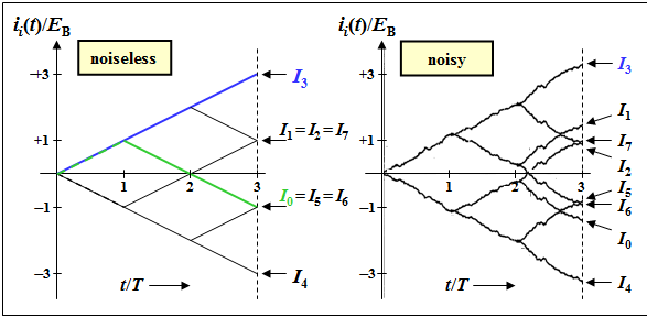
'''(1)''' Die linke Grafik zeigt das Baumdiagramm (ohne Rauschen) mit allen Endwerten. Grün hervorgehoben ist der Verlauf $i_0(t)/E_{\rm B}$ mit dem Endergebnis $I_0/E_{\rm B} = \ –1$, der zunächst linear bis $+1$ ansteigt – das jeweils erste Bit von $s_0(t)$ und $s_3(t)$ stimmen überein – und dann über zwei Bitdauern abfällt.
'''(1)''' The left graph shows the tree diagram (without noise) with all final values. Highlighted in green is the curve $i_0(t)/E_{\rm B}$ with the final result $I_0/E_{\rm B} = \ -1$, which first rises linearly to $+1$ $($the first bit of $s_0(t)$ and $s_3(t)$ in each case coincide$)$ and then falls off over two bit durations.
[[File:EN_Dig_A_3_10_ML.png|right|frame|Tree diagram of the correlation receiver]]
[[File:P_ID1466__Dig_A_3_10.png|center|frame|Baumdiagramm des Korrelationsempfängers]]
'''(2)''' Bei Vorhandensein von (Rausch–) Störungen nehmen die Funktionen $i_i(t)$ nicht mehr linear zu bzw. ab, sondern haben einen Verlauf wie in der oberen Grafik dargestellt. Solange $I_3 > I_{\it i≠3}$ ist, entscheidet der Korrelationsempfänger richtig. Bei Vorhandensein von Störungen gilt stets $I_0 ≠ I_6$ im Gegensatz zum störungsfreien Baumdiagramm. Richtig ist also nur der <u>zweite Lösungsvorschlag</u>.
'''(2)''' Only the <u>second solution</u> is correct:
*In the presence of noises, the functions $i_i(t)$ no longer increase or decrease linearly, but have a curve as shown in the right graph.
*As long as $I_3 > I_{\it i≠3}$, the correlation receiver decides correctly.
*In the presence of noise, $I_0 ≠ I_6$ always holds, in contrast to the noise-free tree diagram.
'''(3)''' Auch hier ist nur die <u>zweite Aussage</u> zutreffend. Da nun die möglichen Sendesignale $s_i(t)$ nicht mehr aus horizontalen Abschnitten zusammengesetzt werden können, besteht auch das Baumdiagramm ohne Störungen nicht aus Geradenstücken. Da die Energien $E_i$ unterschiedlich sind – dies erkennt man zum Beispiel durch den Vergleich der Signale $s_0(t)$ und $s_2(t)$ – müssen für die Entscheidung unbedingt die korrigierten Größen $W_i$ herangezogen werden. Die Verwendung der reinen Korrelationswerte $I_i$ kann bereits ohne Störungen zu Fehlentscheidungen führen.
'''(3)''' Only the <u>second statement</u> is true:
*Since now the possible transmitted signals $s_i(t)$ can no longer be composed of isolated horizontal sections, also the tree diagram without noise does not consist of straight line segments.
*Since the energies $E_i$ are different – this can be seen e.g. by comparing the (red) signals $s_0(t)$ and $s_2(t)$ – it is essential to use the corrected quantities $W_i$ for the decision.
*The use of the uncorrected correlation values $I_i$ can already lead to wrong decisions without noise disturbances.
'''(4)''' Im Fall <u>ohne Impulsinterferenzen</u> (blaue Rechtecksignale) sind alle Signale auf den Bereich $0 \ ... \ 3T$ begrenzt. Außerhalb stellt das Empfangssignal $r(t)$ reines Rauschen dar. Deshalb genügt in diesem Fall auch die Integration über den Bereich $0 \ ... \ 3T$. Richtig ist <u>Antwort 1</u>.
Demgegenüber unterscheiden sich bei Berücksichtigung von Impulsinterferenzen (rote Signale) die Integranden $s_3(t) \cdot s_i(t)$ auch außerhalb dieses Bereichs. Wählt man $t_1 = \ –T$ und $t_2 = +4T$, so wird deshalb die Fehlerwahrscheinlichkeit des Korrelationsempfängers gegenüber dem Integrationsbereich $0 \ ... \ 3T$ weiter verringert.
'''(4)''' <u>Answer 1</u> is correct:
*In the case <u>without intersymbol interference</u> (blue rectangular signals), all signals are limited to the range $0 \ ... \ 3T$.
*Outside this range the received signal $r(t)$ is pure noise. Therefore in this case also the integration over the range $0 \ \text{...} \ 3T$.
*In contrast, when intersymbol interference (red signals) is taken into account, the integrands $s_3(t) \cdot s_i(t)$ also differ outside this range.
*Therefore, if $t_1 = \ -T$ and $t_2 = +4T$ are chosen, the error probability of the correlation receiver is further reduced compared to the integration range $0 \ \text{...} \ 3T$.
{{ML-Fuß}}
{{ML-Fuß}}
Line 80:
Line 97:
[[Category:Aufgaben zu Digitalsignalübertragung|^3.7 Optimale Empfängerstrategien^]]
[[Category:Digital Signal Transmission: Exercises|^3.7 Optimal Receiver Strategies^]]
[[de:Aufgaben:Aufgabe 3.10: Baumdiagramm bei Maximum-Likelihood]]
As in "Exercise 3.9" we consider the joint decision of three binary symbols ("bits") by means of the correlation receiver.
The possible transmitted signals $s_0(t), \ \text{...} \ , \ s_7(t)$ are bipolar.
In the graphic the functions $s_0(t)$, $s_1(t)$, $s_2(t)$ and $s_3(t)$ are shown.
The blue curves are valid for rectangular NRZ transmission pulses.
Below is drawn the so-called "tree diagram" for this constellation under the condition that the signal $s_3(t)$ was sent. Shown here in the range from $0$ to $3T$ are the functions
The correlation receiver compares the final values $I_i = i_i(3T)$ with each other and searches for the largest possible value $I_j$.
The corresponding signal $s_j(t)$ is then the one most likely to have been sent according to the maximum likelihood criterion.
Note that the correlation receiver generally makes the decision based on the corrected quantities
$$W_i = I_i \ - E_i/2.$$
But since for bipolar rectangles all transmitted signals $(i = 0, \ \text{...} \ , \ 7)$ have exactly the same energy
$$E_i = \int_{0}^{3T} s_i^2(t) \,{\rm d} t,$$
the integrals $I_i$ provide exactly the same maximum likelihood information as the corrected quantities $W_i$.
The red signal waveforms $s_i(t)$ are obtained from the blue ones by convolution with the impulse response $h_{\rm G}(t)$ of a Gaussian low-pass filter with cutoff frequency $f_{\rm G} \cdot T = 0.35$.
Each individual rectangular pulse is broadened.
The red signal waveforms lead to "intersymbol interference" in case of threshold decision.
(1) The left graph shows the tree diagram (without noise) with all final values. Highlighted in green is the curve $i_0(t)/E_{\rm B}$ with the final result $I_0/E_{\rm B} = \ -1$, which first rises linearly to $+1$ $($the first bit of $s_0(t)$ and $s_3(t)$ in each case coincide$)$ and then falls off over two bit durations.
Tree diagram of the correlation receiver
In the presence of noises, the functions $i_i(t)$ no longer increase or decrease linearly, but have a curve as shown in the right graph.
As long as $I_3 > I_{\it i≠3}$, the correlation receiver decides correctly.
In the presence of noise, $I_0 ≠ I_6$ always holds, in contrast to the noise-free tree diagram.
(3) Only the second statement is true:
Since now the possible transmitted signals $s_i(t)$ can no longer be composed of isolated horizontal sections, also the tree diagram without noise does not consist of straight line segments.
Since the energies $E_i$ are different – this can be seen e.g. by comparing the (red) signals $s_0(t)$ and $s_2(t)$ – it is essential to use the corrected quantities $W_i$ for the decision.
The use of the uncorrected correlation values $I_i$ can already lead to wrong decisions without noise disturbances.
(4)Answer 1 is correct:
In the case without intersymbol interference (blue rectangular signals), all signals are limited to the range $0 \ ... \ 3T$.
Outside this range the received signal $r(t)$ is pure noise. Therefore in this case also the integration over the range $0 \ \text{...} \ 3T$.
In contrast, when intersymbol interference (red signals) is taken into account, the integrands $s_3(t) \cdot s_i(t)$ also differ outside this range.
Therefore, if $t_1 = \ -T$ and $t_2 = +4T$ are chosen, the error probability of the correlation receiver is further reduced compared to the integration range $0 \ \text{...} \ 3T$.