Difference between revisions of "Aufgaben:Exercise 4.08Z: Error Probability with Three Symbols"
m (Textersetzung - „\*\s*Sollte die Eingabe des Zahlenwertes „0” erforderlich sein, so geben Sie bitte „0\.” ein.“ durch „ “) |
|||
| (8 intermediate revisions by 3 users not shown) | |||
| Line 1: | Line 1: | ||
| − | {{quiz-Header|Buchseite= | + | {{quiz-Header|Buchseite=Digital_Signal_Transmission/Approximation_of_the_Error_Probability}} |
| − | [[File:P_ID2037__Dig_Z_4_8.png|right|frame| | + | [[File:P_ID2037__Dig_Z_4_8.png|right|frame|Decision regions with $M = 3$]] |
| − | + | The diagram shows exactly the same signal space constellation as in [[Aufgaben:Exercise_4.08:_Decision_Regions_at_Three_Symbols|"Exercise 4.8"]]: | |
| − | * | + | * the $M = 3$ possible transmitted signals, viz. |
:$$\boldsymbol{ s }_0 = (-1, \hspace{0.1cm}1)\hspace{0.05cm}, \hspace{0.2cm} | :$$\boldsymbol{ s }_0 = (-1, \hspace{0.1cm}1)\hspace{0.05cm}, \hspace{0.2cm} | ||
\boldsymbol{ s }_1 = (1, \hspace{0.1cm}2)\hspace{0.05cm}, \hspace{0.2cm} | \boldsymbol{ s }_1 = (1, \hspace{0.1cm}2)\hspace{0.05cm}, \hspace{0.2cm} | ||
\boldsymbol{ s }_2 = (2, \hspace{0.1cm}-1)\hspace{0.05cm}.$$ | \boldsymbol{ s }_2 = (2, \hspace{0.1cm}-1)\hspace{0.05cm}.$$ | ||
| − | * | + | * the $M = 3$ decision boundaries |
:$$G_{01}\text{:} \hspace{0.4cm} y \hspace{-0.1cm} \ = \ \hspace{-0.1cm} 1.5 - 2 \cdot x\hspace{0.05cm},$$ | :$$G_{01}\text{:} \hspace{0.4cm} y \hspace{-0.1cm} \ = \ \hspace{-0.1cm} 1.5 - 2 \cdot x\hspace{0.05cm},$$ | ||
:$$G_{02}\text{:} \hspace{0.4cm} y \hspace{-0.1cm} \ = \ \hspace{-0.1cm} -0.75 +1.5 \cdot x\hspace{0.05cm},$$ | :$$G_{02}\text{:} \hspace{0.4cm} y \hspace{-0.1cm} \ = \ \hspace{-0.1cm} -0.75 +1.5 \cdot x\hspace{0.05cm},$$ | ||
| Line 15: | Line 15: | ||
| − | + | The two axes of the two-dimensional signal space are simplistically denoted here as $x$ and $y$; actually, $\varphi_1(t)/\sqrt {E}$ and $\varphi_2(t)/\sqrt {E}$ should be written for these, respectively. | |
| − | + | These decision boundaries are optimal under the two conditions: | |
| − | * | + | * equal probability symbol probabilities, |
| − | |||
| + | * circularly–symmetric PDF of the noise (e.g. AWGN). | ||
| − | In | + | |
| + | In contrast, in this exercise we consider a two–dimensional uniform distribution for the noise PDF: | ||
:$$\boldsymbol{ p }_{\boldsymbol{ n }} (x,\hspace{0.15cm} y) = | :$$\boldsymbol{ p }_{\boldsymbol{ n }} (x,\hspace{0.15cm} y) = | ||
\left\{ \begin{array}{c} K\\ | \left\{ \begin{array}{c} K\\ | ||
0 \end{array} \right.\quad | 0 \end{array} \right.\quad | ||
| − | \begin{array}{*{1}c}{\rm | + | \begin{array}{*{1}c}{\rm for} \hspace{0.15cm}|x| <A, \hspace{0.15cm} |y| <A \hspace{0.05cm}, |
| − | \\ {\rm | + | \\ {\rm else} \hspace{0.05cm}.\\ \end{array}$$ |
| + | |||
| + | *Such an amplitude-limited noise is admittedly without any practical meaning. | ||
| + | |||
| + | *However, it allows an error probability calculation without extensive integrals, from which the principle of the procedure can be seen. | ||
| − | |||
| − | + | Notes: | |
| − | * | + | * The exercise belongs to the chapter [[Digital_Signal_Transmission/Approximation_of_the_Error_Probability|"Approximation of the Error Probability"]]. |
| − | * | + | * To simplify the notation, the following is used: |
:$$x = {\varphi_1(t)}/{\sqrt{E}}\hspace{0.05cm}, \hspace{0.2cm} | :$$x = {\varphi_1(t)}/{\sqrt{E}}\hspace{0.05cm}, \hspace{0.2cm} | ||
y = {\varphi_2(t)}/{\sqrt{E}}\hspace{0.05cm}.$$ | y = {\varphi_2(t)}/{\sqrt{E}}\hspace{0.05cm}.$$ | ||
| Line 42: | Line 46: | ||
| − | === | + | ===Questions=== |
<quiz display=simple> | <quiz display=simple> | ||
| − | { | + | {What is the value of the constant $K$ for $A = 0.75$? |
|type="{}"} | |type="{}"} | ||
$\boldsymbol{K} \ = \ $ { 0.444 3% } | $\boldsymbol{K} \ = \ $ { 0.444 3% } | ||
| − | { | + | {What is the symbol error probability with $A = 0.75$? |
|type="{}"} | |type="{}"} | ||
$p_{\rm S} \ = \ $ { 0. } $\ \%$ | $p_{\rm S} \ = \ $ { 0. } $\ \%$ | ||
| − | { | + | {Which statements are true for $A = 1$? |
|type="[]"} | |type="[]"} | ||
| − | - | + | - All messages $m_i$ are falsified in the same way. |
| − | + | + | + Conditional error probability ${\rm Pr({ \cal E}} \hspace{0.05cm} | \hspace{0.05cm} {\it m}_0) = 1/64$. |
| − | - | + | - Conditional error probability ${\rm Pr({ \cal E}} \hspace{0.05cm} | \hspace{0.05cm} {\it m}_1) = 0$. |
| − | + | + | + Conditional error probability ${\rm Pr({ \cal E}} \hspace{0.05cm} | \hspace{0.05cm} {\it m}_2) = 0$. |
| − | { | + | {What is the error probability with $A=1$ and ${\rm Pr}(m_0) = {\rm Pr}(m_1) = {\rm Pr}(m_2) = 1/3$? |
|type="{}"} | |type="{}"} | ||
$p_{\rm S} \ = \ $ { 1.04 3% } $\ \%$ | $p_{\rm S} \ = \ $ { 1.04 3% } $\ \%$ | ||
| − | { | + | {What is the error probability with $A=1$ and ${\rm Pr}(m_0) = {\rm Pr}(m_1) = 1/4$ and ${\rm Pr}(m_2) = 1/2$? |
|type="{}"} | |type="{}"} | ||
$p_{\rm S} \ = \ $ { 0.78 3% } $\ \%$ | $p_{\rm S} \ = \ $ { 0.78 3% } $\ \%$ | ||
| − | { | + | {Could a better result be obtained by specifying other regions? |
|type="()"} | |type="()"} | ||
| − | + | + | + Yes. |
| − | - | + | - No. |
</quiz> | </quiz> | ||
| − | === | + | ===Solution=== |
{{ML-Kopf}} | {{ML-Kopf}} | ||
| − | '''(1)''' | + | [[File:P_ID2039__Dig_Z_4_8b.png|right|frame|Noise regions with $A = 0.75$]] |
| + | '''(1)''' The volume of the two-dimensional PDF must give $p_n(x, y) =1$, that is: | ||
:$$2A \cdot 2A \cdot K = 1 \hspace{0.3cm}\Rightarrow \hspace{0.3cm} K = \frac{1}{4A^2}\hspace{0.05cm}.$$ | :$$2A \cdot 2A \cdot K = 1 \hspace{0.3cm}\Rightarrow \hspace{0.3cm} K = \frac{1}{4A^2}\hspace{0.05cm}.$$ | ||
| − | + | *With $A = 0.75$ ⇒ $2A = 3/2$, we get $K = 4/9 \ \underline {=0.444}$. | |
| + | |||
| − | + | '''(2)''' In the accompanying graph, the noise component $\boldsymbol{n}$ is plotted by the squares of edge length $1.5$ around the signal space points $\boldsymbol{s}_i$. | |
| − | '''(2)''' In | + | *It can be seen that no decision boundary is exceeded by noise components. |
| + | *It follows: The symbol error probability is $p_{\rm S}\ \underline { \equiv 0}$ under the conditions given here. | ||
| + | <br clear=all> | ||
| + | [[File:P_ID2040__Dig_Z_4_8c.png|right|frame|Noise regions with $A = 1$]] | ||
| + | '''(3)''' <u>Statements 2 and 4</u> are correct, as can be seen from the second graph: | ||
| + | * The message $m_2$ cannot be falsified because the square around $\boldsymbol{s}_2$ lies entirely in the lower right quadrant and thus in the decision region $I_2$. | ||
| − | + | * Likewise, $m_2$ was sent with certainty if the received value lies in decision region $I_2$. <br>The reason: None of the squares around $\boldsymbol{s}_0$ and $\boldsymbol{s}_1$ extends into the region $I_2$. | |
| − | + | ||
| − | + | * $m_0$ can only be falsified to $m_1$. The (conditional) falsification probability is equal to the ratio of the areas of the small yellow triangle $($area $1/16)$ and the square $($area $4)$: | |
| − | * $m_0$ | ||
| − | |||
:$${\rm Pr}({ \cal E}\hspace{0.05cm}|\hspace{0.05cm} m_0 ) = \frac{1/2 \cdot 1/2 \cdot 1/4}{4}= {1}/{64} | :$${\rm Pr}({ \cal E}\hspace{0.05cm}|\hspace{0.05cm} m_0 ) = \frac{1/2 \cdot 1/2 \cdot 1/4}{4}= {1}/{64} | ||
\hspace{0.05cm}.$$ | \hspace{0.05cm}.$$ | ||
| − | * | + | * For symmetry reasons, equally: |
:$${\rm Pr}({ \cal E}\hspace{0.05cm}|\hspace{0.05cm} m_1 ) = {\rm Pr}({ \cal E}\hspace{0.05cm}|\hspace{0.05cm} m_0 )={1}/{64} | :$${\rm Pr}({ \cal E}\hspace{0.05cm}|\hspace{0.05cm} m_1 ) = {\rm Pr}({ \cal E}\hspace{0.05cm}|\hspace{0.05cm} m_0 )={1}/{64} | ||
\hspace{0.05cm}. $$ | \hspace{0.05cm}. $$ | ||
| − | '''(4)''' | + | '''(4)''' For equal probability symbols, we obtain for the (average) error probability: |
| − | :$$p_{\rm S} = {\rm Pr}({ \cal E} ) = {1}/{3} \cdot \ | + | :$$p_{\rm S} = {\rm Pr}({ \cal E} ) = {1}/{3} \cdot \big [{\rm Pr}({ \cal E}\hspace{0.05cm}|\hspace{0.05cm} m_0 ) + {\rm Pr}({ \cal E}\hspace{0.05cm}|\hspace{0.05cm} m_1 )+{\rm Pr}({ \cal E}\hspace{0.05cm}|\hspace{0.05cm} m_2 )\big ]$$ |
:$$ \Rightarrow \hspace{0.3cm} p_{\rm S} = {\rm Pr}({ \cal E} ) = {1}/{3} \cdot \left [{1}/{64} + {1}/{64} + 0 )\right ]= \frac{2}{3 \cdot 64} = {1}/{96}\hspace{0.1cm}\hspace{0.15cm}\underline {\approx 1.04 \%} \hspace{0.05cm}.$$ | :$$ \Rightarrow \hspace{0.3cm} p_{\rm S} = {\rm Pr}({ \cal E} ) = {1}/{3} \cdot \left [{1}/{64} + {1}/{64} + 0 )\right ]= \frac{2}{3 \cdot 64} = {1}/{96}\hspace{0.1cm}\hspace{0.15cm}\underline {\approx 1.04 \%} \hspace{0.05cm}.$$ | ||
| − | '''(5)''' | + | '''(5)''' Now we obtain a smaller average error probability, viz. |
:$$p_{\rm S} = {\rm Pr}({ \cal E} ) = {1}/{4} \cdot {1}/{64} + {1}/{4} \cdot {1}/{64}+ {1}/{2} \cdot0 = {1}/{128}\hspace{0.1cm}\hspace{0.15cm}\underline {\approx 0.78 \% } \hspace{0.05cm}. $$ | :$$p_{\rm S} = {\rm Pr}({ \cal E} ) = {1}/{4} \cdot {1}/{64} + {1}/{4} \cdot {1}/{64}+ {1}/{2} \cdot0 = {1}/{128}\hspace{0.1cm}\hspace{0.15cm}\underline {\approx 0.78 \% } \hspace{0.05cm}. $$ | ||
| − | '''(6)''' <u> | + | '''(6)''' <u>Correct is YES</u>: |
| − | * | + | *For example, $I_1$: first quadrant, $I_0$: second quadrant, $I_2 \text{:} \ y < 0$ would give zero error probability. |
| − | * | + | |
| + | *This means that the given bounds are optimal only in the case of circularly symmetric PDF of the noise, for example, the AWGN model. | ||
{{ML-Fuß}} | {{ML-Fuß}} | ||
| − | [[Category: | + | [[Category:Digital Signal Transmission: Exercises|^4.3 BER Approximation^]] |
Latest revision as of 18:16, 28 July 2022
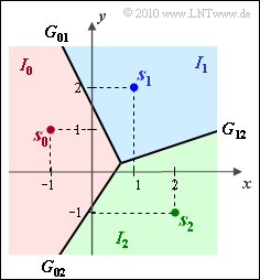
The diagram shows exactly the same signal space constellation as in "Exercise 4.8":
- the $M = 3$ possible transmitted signals, viz.
- $$\boldsymbol{ s }_0 = (-1, \hspace{0.1cm}1)\hspace{0.05cm}, \hspace{0.2cm} \boldsymbol{ s }_1 = (1, \hspace{0.1cm}2)\hspace{0.05cm}, \hspace{0.2cm} \boldsymbol{ s }_2 = (2, \hspace{0.1cm}-1)\hspace{0.05cm}.$$
- the $M = 3$ decision boundaries
- $$G_{01}\text{:} \hspace{0.4cm} y \hspace{-0.1cm} \ = \ \hspace{-0.1cm} 1.5 - 2 \cdot x\hspace{0.05cm},$$
- $$G_{02}\text{:} \hspace{0.4cm} y \hspace{-0.1cm} \ = \ \hspace{-0.1cm} -0.75 +1.5 \cdot x\hspace{0.05cm},$$
- $$G_{12}\text{:} \hspace{0.4cm} y \hspace{-0.1cm} \ = \ \hspace{-0.1cm} x/3\hspace{0.05cm}.$$
The two axes of the two-dimensional signal space are simplistically denoted here as $x$ and $y$; actually, $\varphi_1(t)/\sqrt {E}$ and $\varphi_2(t)/\sqrt {E}$ should be written for these, respectively.
These decision boundaries are optimal under the two conditions:
- equal probability symbol probabilities,
- circularly–symmetric PDF of the noise (e.g. AWGN).
In contrast, in this exercise we consider a two–dimensional uniform distribution for the noise PDF:
- $$\boldsymbol{ p }_{\boldsymbol{ n }} (x,\hspace{0.15cm} y) = \left\{ \begin{array}{c} K\\ 0 \end{array} \right.\quad \begin{array}{*{1}c}{\rm for} \hspace{0.15cm}|x| <A, \hspace{0.15cm} |y| <A \hspace{0.05cm}, \\ {\rm else} \hspace{0.05cm}.\\ \end{array}$$
- Such an amplitude-limited noise is admittedly without any practical meaning.
- However, it allows an error probability calculation without extensive integrals, from which the principle of the procedure can be seen.
Notes:
- The exercise belongs to the chapter "Approximation of the Error Probability".
- To simplify the notation, the following is used:
- $$x = {\varphi_1(t)}/{\sqrt{E}}\hspace{0.05cm}, \hspace{0.2cm} y = {\varphi_2(t)}/{\sqrt{E}}\hspace{0.05cm}.$$
Questions
Solution
(1) The volume of the two-dimensional PDF must give $p_n(x, y) =1$, that is:
- $$2A \cdot 2A \cdot K = 1 \hspace{0.3cm}\Rightarrow \hspace{0.3cm} K = \frac{1}{4A^2}\hspace{0.05cm}.$$
- With $A = 0.75$ ⇒ $2A = 3/2$, we get $K = 4/9 \ \underline {=0.444}$.
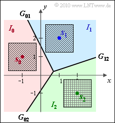
(2) In the accompanying graph, the noise component $\boldsymbol{n}$ is plotted by the squares of edge length $1.5$ around the signal space points $\boldsymbol{s}_i$.
- It can be seen that no decision boundary is exceeded by noise components.
- It follows: The symbol error probability is $p_{\rm S}\ \underline { \equiv 0}$ under the conditions given here.
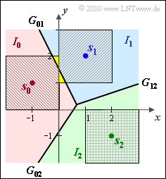
(3) Statements 2 and 4 are correct, as can be seen from the second graph:
- The message $m_2$ cannot be falsified because the square around $\boldsymbol{s}_2$ lies entirely in the lower right quadrant and thus in the decision region $I_2$.
- Likewise, $m_2$ was sent with certainty if the received value lies in decision region $I_2$.
The reason: None of the squares around $\boldsymbol{s}_0$ and $\boldsymbol{s}_1$ extends into the region $I_2$.
- $m_0$ can only be falsified to $m_1$. The (conditional) falsification probability is equal to the ratio of the areas of the small yellow triangle $($area $1/16)$ and the square $($area $4)$:
- $${\rm Pr}({ \cal E}\hspace{0.05cm}|\hspace{0.05cm} m_0 ) = \frac{1/2 \cdot 1/2 \cdot 1/4}{4}= {1}/{64} \hspace{0.05cm}.$$
- For symmetry reasons, equally:
- $${\rm Pr}({ \cal E}\hspace{0.05cm}|\hspace{0.05cm} m_1 ) = {\rm Pr}({ \cal E}\hspace{0.05cm}|\hspace{0.05cm} m_0 )={1}/{64} \hspace{0.05cm}. $$
(4) For equal probability symbols, we obtain for the (average) error probability:
- $$p_{\rm S} = {\rm Pr}({ \cal E} ) = {1}/{3} \cdot \big [{\rm Pr}({ \cal E}\hspace{0.05cm}|\hspace{0.05cm} m_0 ) + {\rm Pr}({ \cal E}\hspace{0.05cm}|\hspace{0.05cm} m_1 )+{\rm Pr}({ \cal E}\hspace{0.05cm}|\hspace{0.05cm} m_2 )\big ]$$
- $$ \Rightarrow \hspace{0.3cm} p_{\rm S} = {\rm Pr}({ \cal E} ) = {1}/{3} \cdot \left [{1}/{64} + {1}/{64} + 0 )\right ]= \frac{2}{3 \cdot 64} = {1}/{96}\hspace{0.1cm}\hspace{0.15cm}\underline {\approx 1.04 \%} \hspace{0.05cm}.$$
(5) Now we obtain a smaller average error probability, viz.
- $$p_{\rm S} = {\rm Pr}({ \cal E} ) = {1}/{4} \cdot {1}/{64} + {1}/{4} \cdot {1}/{64}+ {1}/{2} \cdot0 = {1}/{128}\hspace{0.1cm}\hspace{0.15cm}\underline {\approx 0.78 \% } \hspace{0.05cm}. $$
(6) Correct is YES:
- For example, $I_1$: first quadrant, $I_0$: second quadrant, $I_2 \text{:} \ y < 0$ would give zero error probability.
- This means that the given bounds are optimal only in the case of circularly symmetric PDF of the noise, for example, the AWGN model.


