Aufgaben:Exercise 1.2: Lognormal Channel Model: Difference between revisions

From LNTwww
No edit summary
Fix interlanguage link: resolve redirect chain
 
(22 intermediate revisions by 5 users not shown)
Line 1: Line 1:
{{quiz-Header|Buchseite=Mobile Kommunikation/Distanzabhängige Dämpfung und Abschattung
{{quiz-Header|Buchseite=Mobile_Communications/Distance_Dependent_Attenuation_and_Shading
}}
}}


[[File:P_ID2122__Mob_A_1_2.png|right|frame|PDF of lognormal fading]]
[[File:EN_Mob_A1_2.png|right|frame|PDF of lognormal fading]]
We consider a mobile radio cell in an urban area and a vehicle that is approximately at a fixed distance  $d_0$  from the base station. For example, it moves on an arc around the base station.  
We consider a mobile radio cell in an urban area and a vehicle that is approximately at a fixed distance  $d_0$  from the base station.  For example, it moves on an arc around the base station.  


Thus the total path loss can be described by the following equation:
$$V_{\rm P} = V_{\rm 0} + V_{\rm S}  \hspace{0.05cm}.$$
:$$V_{\rm P} = V_{\rm 0} + V_{\rm S}  \hspace{0.05cm}.$$


*$V_0$  takes into account the distance-dependent path loss which is assumed to be constant: $V_0 = 80 \ \rm dB$ .  
*$V_0$  takes into account the distance-dependent path loss which is assumed to be constant:  $V_0 = 80 \ \rm dB$ .  
*The loss  $V_{\rm S}$  is due to shadowing caused by the lognormal–distribution with the probability density function (PDF)
*The loss  $V_{\rm S}$  is due to shadowing caused by the lognormal distribution with the probability density function (PDF)
:$$f_{V{\rm S}}(V_{\rm S}) =  \frac {1}{ \sqrt{2 \pi }\cdot \sigma_{\rm S}}  \cdot {\rm exp } \left [ - \frac{ (V_{\rm S}- m_{\rm S})^2}{2 \cdot \sigma_{\rm S}^2} \right ] \hspace{0.05cm}$$
:$$f_{V_{\rm S}}(V_{\rm S}) =  \frac {1}{ \sqrt{2 \pi }\cdot \sigma_{\rm S}}  \cdot {\rm e }^{ - { (V_{\rm S}\hspace{0.05cm}- \hspace{0.05cm}m_{\rm S})^2}/(2 \hspace{0.05cm}\cdot \hspace{0.05cm}\sigma_{\rm S}^2) },$$


: see diagram. The following numerical values apply:
$$m_{\rm S} = 20\,\,{\rm dB}\hspace{0.05cm},\hspace{0.2cm}  \sigma_{\rm S} = 10\,\,{\rm dB}\hspace{0.15cm}{\rm or }\hspace{0.15cm}\sigma_{\rm S} = 0\,\,{\rm dB}\hspace{0.15cm}{\rm (subtask\hspace{0.15cm} 2)}\hspace{0.05cm}.$$
:$$m_{\rm S} = 20\,\,{\rm dB}\hspace{0.05cm},\hspace{0.2cm}  \sigma_{\rm S} = 10\,\,{\rm dB}\hspace{0.25cm}{\rm or }\hspace{0.25cm}\sigma_{\rm S} = 0\,\,{\rm dB}\hspace{0.15cm}{\rm (subtask\hspace{0.15cm} 2)}\hspace{0.05cm}.$$


Also make the following simple assumptions:
* The transmit power is  $P_{\rm S} = 10 \ \rm W$  (or $40 \ \rm dBm$).
* The transmit power is  $P_{\rm S} = 10 \ \rm W$  $\text{(or } 40 \ \rm dBm$).
* The receive power should be at least  $P_{\rm E} = 10 \ \rm pW$  (or $–80 \ \rm dBm$)
* The received power should be at least  $P_{\rm E} = 10 \ \rm pW$  $\text{(or } -80 \ \rm dBm$)


Line 25: Line 25:


Notes:''  
Notes:''  
* This task belongs to the chapter  [[Mobile_Kommunikation/Distanzabh%C3%A4ngige_D%C3%A4mpfung_und_Abschattung|Distanzabhängige Dämpfung und Abschattung]].
* This task belongs to the chapter  [[Mobile_Communications/Distance_dependent_attenuation_and_shading|Distance dependent attenuation and shading]].
   
   
* You can use the following (rough) approximations for the complementary Gaussian error integral:
:$${\rm Q}(1) \approx 0.16\hspace{0.05cm},\hspace{0.2cm} {\rm Q}(2) \approx 0.02\hspace{0.05cm},\hspace{0.2cm}
:$${\rm Q}(1) \approx 0.16\hspace{0.05cm},\hspace{0.2cm} {\rm Q}(2) \approx 0.02\hspace{0.05cm},\hspace{0.2cm}{\rm Q}(3) \approx 10^{-3}\hspace{0.05cm}.$$
{\rm Q}(3) \approx 10^{-3}\hspace{0.05cm}.$$
* Or use the interaction module  [[Applets:Complementary_Gaussian_Error_Functions|Complementary Gaussian Error Functions]]  provided by  $\rm LNTwww$.
* Or use the interaction module provided by $\rm LNTwww$ [[Applets:Komplementäre_Gaußsche_Fehlerfunktionen_(neues_Applet)|Komplementäre Gaußsche Fehlerfunktionen]].


===Questionnaire===
===Questions===


<quiz display=simple>
{Would&nbsp; $P_{\rm E}$&nbsp; without consideration of the lognormal&ndash;fading be sufficient?
{Would&nbsp; $P_{\rm E}$&nbsp; be sufficient if the loss $V_S$ due to shadowing is not present?
|type="()"}
|type="()"}
+ Yes,
+ Yes,
- No.
- No.


{The parameters of the lognormal distribution are&nbsp; $m_{\rm S} = 20 \, \rm dB$&nbsp; and&nbsp; $\sigma_{\rm S} = 0 \, \rm dB$. What percentage of the time does the system work?
{The parameters of the lognormal distribution are&nbsp; $m_{\rm S} = 20 \, \rm dB$&nbsp; and&nbsp; $\sigma_{\rm S} = 0 \, \rm dB$.&nbsp; What percentage of the time does the system work?
|type="{}"}
|type="{}"}
${\rm Pr(System \ works)} \ = \ $ { 100 3% } $\ \%$
Line 50: Line 49:
${\rm Pr(System \ works)}\ = \ $ { 98 3% } $\ \%$


{How big can&nbsp; $V_0$&nbsp; be at most, so that the reliability of &nbsp; $99.9\%$&nbsp; is reached?
{How big can&nbsp; $V_0$&nbsp; be at most, so that the reliability of&nbsp; $99.9\%$&nbsp; is reached?
|type="{}"}
|type="{}"}
$V_0 \ = \ $ { 70 3% } $\ \ \rm dB$
</quiz>
</quiz>


===Sample solution===
===Solution===
{{ML-Kopf}}
{{ML-Kopf}}
'''(1)'''&nbsp; The correct answer is <u>YES</u>:
*From the $\rm dB$&ndash;value $V_0 = 80 \ \rm dB$ follows the absolute (linear) value $K_0 = 10^8$. Thus the received power is
*From the&nbsp; $\rm dB$&ndash;value&nbsp; $V_0 = 80 \ \rm dB$&nbsp; follows the absolute (linear) value&nbsp; $K_0 = 10^8$.&nbsp; Thus the received power is
$$P_{\rm E} = P_{\rm S}/K_0 = 10 \ {\rm W}/10^8 = 100 \ {\rm nW} > 10 \ \ \rm pW.$$  
:$$P_{\rm E} = P_{\rm S}/K_0 = 10 \ {\rm W}/10^8 = 100 \ {\rm nW} > 10 \ \ \rm pW.$$  


*You can also solve this problem directly with the logarithmic quantities:
:$$10 \cdot {\rm lg}\hspace{0.15cm} \frac{P_{\rm E}}{1\,\,{\rm mW}} = 10 \cdot {\rm lg}\hspace{0.15cm} \frac{P_{\rm S}}{1\,\,{\rm mW}} - V_0 = 40\,{\rm dBm} -80\,\,{\rm dB} = -40\,\,{\rm dBm}  
:$$10 \cdot {\rm lg}\hspace{0.15cm} \frac{P_{\rm E}}{1\,\,{\rm mW}} = 10 \cdot {\rm lg}\hspace{0.15cm} \frac{P_{\rm S}}{1\,\,{\rm mW}} - V_0 = 40\,{\rm dBm} -80\,\,{\rm dB} = -40\,\,{\rm dBm}\hspace{0.05cm}.$$
  \hspace{0.05cm}.$$


*Only the limit value $&ndash;80 \ \rm dBm$ is required.
*Only the limit value&nbsp; $-80 \ \rm dBm$&nbsp; is required.


'''(2)'''&nbsp; Lognormal&ndash;Fading with $\sigma_{\rm S} = 0 \ \rm dB$ is equivalent to a constant receive power $P_{\rm E}$.  
'''(2)'''&nbsp; Lognormal fading with&nbsp; $\sigma_{\rm S} = 0 \ \rm dB$&nbsp; is equivalent to a constant received power&nbsp; $P_{\rm E}$.  
*Compared to the subtask '''(1)'' this is $m_{\rm S} = 20 \ \ \rm dB$ smaller &nbsp; &#8658; &nbsp; $P_{\rm E} = \ &ndash;60 \ \ \rm dBm$.  
*Compared to the subtask&nbsp; '''(1)'''&nbsp; this is&nbsp; $m_{\rm S} = 20 \ \ \rm dB$&nbsp; smaller &nbsp; &#8658; &nbsp; $P_{\rm E} = \ &ndash;60 \ \ \rm dBm$.  
*But it is still greater than the specified limit value ($&ndash;80 \ \rm dBm$).  
*But it is still greater than the specified limit value&nbsp; $(-80 \ \rm dBm)$.  
*It follows: &nbsp; The system is (almost) <u>100% functional</u>. &bdquo;Almost&rdquo; because with a Gaussian random quantity there is always a (small) residual uncertainty.
*It follows: &nbsp; The system is (almost)&nbsp; <u>100% functional</u>.&nbsp; "Almost" because with a Gaussian random quantity there is always a (small) residual uncertainty.


'''(3)'''&nbsp; The receive power is too low (less than $&ndash;80 \ \rm dBm$) if the power loss due to the lognormal&ndash;term is $40 \ \rm dB$ or more.  
'''(3)'''&nbsp; The received power is too low&nbsp; $($less than $&ndash;80 \ \rm dBm)$&nbsp; if the power loss due to the lognormal&ndash;term is&nbsp; $40 \ \rm dB$&nbsp; or more.
*The variable portion $V_{\rm S}$ must therefore not be greater than $20 \ \rm dB$.  
[[File:EN_Mob_A_1_2c.png|right|frame|Loss due to lognormal fading]]
*The distance-dependent path loss $V_{\rm S}$ must therefore not be greater than&nbsp; $20 \ \rm dB$.  
*So it follows:
*So it follows:
:$${\rm Pr}({\rm "System\hspace{0.15cm}does\hspace{0.15cm}not\hspace{0.15cm}work"})= {\rm Q}\left ( \frac{20\,\,{\rm dB}}{\sigma_{\rm S} = 10\,{\rm dB}}\right )  
:$${\rm Pr}({\rm "System\hspace{0.15cm}does\hspace{0.15cm}not\hspace{0.15cm}work"})= {\rm Q}\left ( \frac{20\,\,{\rm dB}}{\sigma_{\rm S} = 10\,{\rm dB}}\right )= {\rm Q}(2) \approx 0.02$$
  = {\rm Q}(2) \approx 0.02\hspace{0.3cm}
:$$\Rightarrow \hspace{0.3cm}{\rm Pr}({\rm "System\hspace{0.15cm}works"})= 1-  0.02 \hspace{0.15cm} \underline{\approx 98\,\%}\hspace{0.05cm}.$$
\Rightarrow \hspace{0.3cm}{\rm Pr}({\rm "System\hspace{0.15cm}works"})= 1-  0.02 \hspace{0.15cm} \underline{\approx 98\,\%}\hspace{0.05cm}.$$
[[File:P_ID2187__Mob_A_1_2c_v1.png|right|frame|loss due to lognormal fading]]
The graphic illustrates the result.  
*The probability density $f_{\rm VS}(V_{\rm S})$ of the path loss due to shadowing (Longnormal&ndash;Fading) is shown here.  
*The probability density&nbsp; $f_{\rm VS}(V_{\rm S})$&nbsp; of the path loss due to shadowing&nbsp; (Longnormal Fading)&nbsp; is shown here.  
 
*The probability that the system will fail is marked in red.


*The probability that the system will fail is marked in red:
'''(4)'''&nbsp; From the availability probability&nbsp; $99.9 \%$&nbsp; follows the failure probability&nbsp; $10^{\rm -3} \approx \ {\rm Q}(3)$.  
<br clear=all>
*If the distance-dependent path loss&nbsp; $V_0$&nbsp; is reduced by&nbsp; $10 \ \ \rm dB$&nbsp; to&nbsp; $\underline {70 \ \rm dB}$, a failure will only occur when&nbsp; $V_{\rm S} &#8805; 50 \ \ \rm dB$.  
'''(4)'''&nbsp; From the availability probability $99.9 \%$ follows the failure probability $10^{\rm &ndash;3} \approx \ {\rm Q}(3)$.  
*If the distance-dependent path loss $V_0$ is reduced by $10 \ \ \rm dB$ to $\underline {70 \ \rm dB}$, a failure will only occur when $V_{\rm S} &#8805; 50 \ \ \rm dB$.  
*This would achieve exactly the required reliability, as the following calculation shows:  
$${\rm Pr}({\rm "System\hspace{0.15cm} does not work\hspace{0.15cm}"})=
:$${\rm Pr}({\rm "System\hspace{0.15cm} does\hspace{0.15cm} not\hspace{0.15cm} work\hspace{0.15cm}"})={\rm Q}\left ( \frac{120-70-20}{10}\right )= {\rm Q}(3) \approx 0.001 \hspace{0.05cm}.$$
  {\rm Q}\left ( \frac{120-70-20}{10}\right )  
  = {\rm Q}(3) \approx 0.001 \hspace{0.05cm}.$$


{{ML-Fuß}}
{{ML-Fuß}}
Line 102: Line 100:


[[Category:Exercises for Mobile Communications|^1.1 Distance-dependent attenuation^]]
[[Category:Mobile Communications: Exercises|^1.1 Distance-Dependent Attenuation^]]
[[de:Aufgaben:Exercise 1.2: Lognormal Channel Model]]

Latest revision as of 17:54, 16 March 2026

PDF of lognormal fading

We consider a mobile radio cell in an urban area and a vehicle that is approximately at a fixed distance  $d_0$  from the base station.  For example, it moves on an arc around the base station.

Thus the total path loss can be described by the following equation:

$$V_{\rm P} = V_{\rm 0} + V_{\rm S} \hspace{0.05cm}.$$
  • $V_0$  takes into account the distance-dependent path loss which is assumed to be constant:  $V_0 = 80 \ \rm dB$ .
  • The loss  $V_{\rm S}$  is due to shadowing caused by the lognormal distribution with the probability density function (PDF)
$$f_{V_{\rm S}}(V_{\rm S}) = \frac {1}{ \sqrt{2 \pi }\cdot \sigma_{\rm S}} \cdot {\rm e }^{ - { (V_{\rm S}\hspace{0.05cm}- \hspace{0.05cm}m_{\rm S})^2}/(2 \hspace{0.05cm}\cdot \hspace{0.05cm}\sigma_{\rm S}^2) },$$
see diagram. The following numerical values apply:
$$m_{\rm S} = 20\,\,{\rm dB}\hspace{0.05cm},\hspace{0.2cm} \sigma_{\rm S} = 10\,\,{\rm dB}\hspace{0.25cm}{\rm or }\hspace{0.25cm}\sigma_{\rm S} = 0\,\,{\rm dB}\hspace{0.15cm}{\rm (subtask\hspace{0.15cm} 2)}\hspace{0.05cm}.$$

Also make the following simple assumptions:

  • The transmit power is  $P_{\rm S} = 10 \ \rm W$  $\text{(or } 40 \ \rm dBm$).
  • The received power should be at least  $P_{\rm E} = 10 \ \rm pW$  $\text{(or } -80 \ \rm dBm$)


Notes:

  • You can use the following (rough) approximations for the complementary Gaussian error integral:
$${\rm Q}(1) \approx 0.16\hspace{0.05cm},\hspace{0.2cm} {\rm Q}(2) \approx 0.02\hspace{0.05cm},\hspace{0.2cm}{\rm Q}(3) \approx 10^{-3}\hspace{0.05cm}.$$


Questions

1 Would  $P_{\rm E}$  be sufficient if the loss $V_S$ due to shadowing is not present?

Yes,
No.

2 The parameters of the lognormal distribution are  $m_{\rm S} = 20 \, \rm dB$  and  $\sigma_{\rm S} = 0 \, \rm dB$.  What percentage of the time does the system work?

${\rm Pr(System \ works)} \ = \ $ $\ \%$

3 What is the probability with  $m_{\rm S} = 20 \ \ \rm dB$  and  $\sigma_{\rm S} = 10 \ \ \rm dB$?

${\rm Pr(System \ works)}\ = \ $ $\ \%$

4 How big can  $V_0$  be at most, so that the reliability of  $99.9\%$  is reached?

$V_0 \ = \ $ $\ \ \rm dB$


Solution

(1)  The correct answer is YES:

  • From the  $\rm dB$–value  $V_0 = 80 \ \rm dB$  follows the absolute (linear) value  $K_0 = 10^8$.  Thus the received power is
$$P_{\rm E} = P_{\rm S}/K_0 = 10 \ {\rm W}/10^8 = 100 \ {\rm nW} > 10 \ \ \rm pW.$$
  • You can also solve this problem directly with the logarithmic quantities:
$$10 \cdot {\rm lg}\hspace{0.15cm} \frac{P_{\rm E}}{1\,\,{\rm mW}} = 10 \cdot {\rm lg}\hspace{0.15cm} \frac{P_{\rm S}}{1\,\,{\rm mW}} - V_0 = 40\,{\rm dBm} -80\,\,{\rm dB} = -40\,\,{\rm dBm}\hspace{0.05cm}.$$
  • Only the limit value  $-80 \ \rm dBm$  is required.


(2)  Lognormal fading with  $\sigma_{\rm S} = 0 \ \rm dB$  is equivalent to a constant received power  $P_{\rm E}$.

  • Compared to the subtask  (1)  this is  $m_{\rm S} = 20 \ \ \rm dB$  smaller   ⇒   $P_{\rm E} = \ –60 \ \ \rm dBm$.
  • But it is still greater than the specified limit value  $(-80 \ \rm dBm)$.
  • It follows:   The system is (almost)  100% functional.  "Almost" because with a Gaussian random quantity there is always a (small) residual uncertainty.


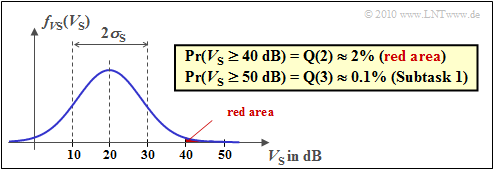
(3)  The received power is too low  $($less than $–80 \ \rm dBm)$  if the power loss due to the lognormal–term is  $40 \ \rm dB$  or more.

Loss due to lognormal fading
  • The distance-dependent path loss $V_{\rm S}$ must therefore not be greater than  $20 \ \rm dB$.
  • So it follows:
$${\rm Pr}({\rm "System\hspace{0.15cm}does\hspace{0.15cm}not\hspace{0.15cm}work"})= {\rm Q}\left ( \frac{20\,\,{\rm dB}}{\sigma_{\rm S} = 10\,{\rm dB}}\right )= {\rm Q}(2) \approx 0.02$$
$$\Rightarrow \hspace{0.3cm}{\rm Pr}({\rm "System\hspace{0.15cm}works"})= 1- 0.02 \hspace{0.15cm} \underline{\approx 98\,\%}\hspace{0.05cm}.$$

The graphic illustrates the result.

  • The probability density  $f_{\rm VS}(V_{\rm S})$  of the path loss due to shadowing  (Longnormal Fading)  is shown here.
  • The probability that the system will fail is marked in red.


(4)  From the availability probability  $99.9 \%$  follows the failure probability  $10^{\rm -3} \approx \ {\rm Q}(3)$.

  • If the distance-dependent path loss  $V_0$  is reduced by  $10 \ \ \rm dB$  to  $\underline {70 \ \rm dB}$, a failure will only occur when  $V_{\rm S} ≥ 50 \ \ \rm dB$.
  • This would achieve exactly the required reliability, as the following calculation shows:
$${\rm Pr}({\rm "System\hspace{0.15cm} does\hspace{0.15cm} not\hspace{0.15cm} work\hspace{0.15cm}"})={\rm Q}\left ( \frac{120-70-20}{10}\right )= {\rm Q}(3) \approx 0.001 \hspace{0.05cm}.$$