Difference between revisions of "Aufgaben:Exercise 4.1: Low-Pass and Band-Pass Signals"
| (10 intermediate revisions by 3 users not shown) | |||
| Line 3: | Line 3: | ||
}} | }} | ||
| − | [[File:P_ID691__Sig_A_4_1.png|250px|right|frame| | + | [[File:P_ID691__Sig_A_4_1.png|250px|right|frame|Given signal curves]] |
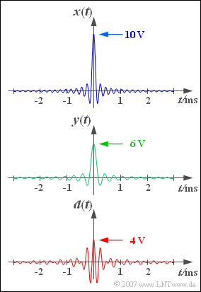
Three signal curves are sketched on the right, the first two having the following curve: | Three signal curves are sketched on the right, the first two having the following curve: | ||
| Line 13: | Line 13: | ||
{t}/{T_y}) .$$ | {t}/{T_y}) .$$ | ||
| − | $T_x = 100 \,{\rm µ}\text{s}$ and $T_y = 166.67 \,{\rm µ}\text{s}$ indicate the first zero of $x(t)$ | + | $T_x = 100 \,{\rm µ}\text{s}$ and $T_y = 166.67 \,{\rm µ}\text{s}$ indicate the first zero of $x(t)$ and $y(t)$ respectively. |
The signal $d(t)$ results from the difference of the two upper signals (lower graph): | The signal $d(t)$ results from the difference of the two upper signals (lower graph): | ||
| − | |||
:$$d(t) = x(t)-y(t) .$$ | :$$d(t) = x(t)-y(t) .$$ | ||
| − | In | + | In subtask '''(4)''' the integral areas of the pulses $x(t)$ and $d(t)$ are asked for. For these holds: |
:$$F_x = \int_{- \infty}^{+\infty}\hspace{-0.4cm}x(t)\hspace{0.1cm}{\rm d}t , \hspace{0.5cm}F_d = \int_{- \infty}^{+\infty}\hspace{-0.4cm}d(t)\hspace{0.1cm}{\rm d}t .$$ | :$$F_x = \int_{- \infty}^{+\infty}\hspace{-0.4cm}x(t)\hspace{0.1cm}{\rm d}t , \hspace{0.5cm}F_d = \int_{- \infty}^{+\infty}\hspace{-0.4cm}d(t)\hspace{0.1cm}{\rm d}t .$$ | ||
| Line 41: | Line 40: | ||
''Hints:'' | ''Hints:'' | ||
| − | *This exercise belongs to the chapter [[Signal_Representation/ | + | *This exercise belongs to the chapter [[Signal_Representation/Differences_and_Similarities_of_Low-Pass_and_Band-Pass_Signals|Differences and Similarities of Low-Pass and Band-Pass Signals]]. |
| − | *The Fourier | + | *The inverse Fourier transform of a rectangular spectrum $X(f)$ leads to an $\rm si$–shaped time function $x(t)$: |
:$$X(f)=\left\{ {X_0 \; \rm f\ddot{u}r\; |\it f| < \rm B, \atop {\rm 0 \;\;\; \rm sonst}}\right. \;\; | :$$X(f)=\left\{ {X_0 \; \rm f\ddot{u}r\; |\it f| < \rm B, \atop {\rm 0 \;\;\; \rm sonst}}\right. \;\; | ||
\bullet\!\!-\!\!\!-\!\!\!-\!\!\circ\, \;\;x(t) = 2 \cdot X_0 \cdot B \cdot {\rm si} ( 2\pi B t) .$$ | \bullet\!\!-\!\!\!-\!\!\!-\!\!\circ\, \;\;x(t) = 2 \cdot X_0 \cdot B \cdot {\rm si} ( 2\pi B t) .$$ | ||
| − | *In this task, the function $\rm si(x) = \rm sin(x)/x = \rm sinc(x/π)$ is used. | + | *In this task, the function $\rm si(x) = \rm sin(x)/x = \rm sinc(x/π)$ is used. |
| Line 54: | Line 53: | ||
<quiz display=simple> | <quiz display=simple> | ||
| − | {What is the spectrum $X(f)$ of the signal $x(t)$? What are the magnitudes of $X(f = 0)$ and the physical, one-sided bandwidth $B_x$ of $x(t)$? | + | {What is the spectrum $X(f)$ of the signal $x(t)$? What are the magnitudes of $X(f = 0)$ and the physical, one-sided bandwidth $B_x$ of $x(t)$? |
|type="{}"} | |type="{}"} | ||
$X(f=0)\ = \ $ { 1 3% } $\text{mV/Hz}$ | $X(f=0)\ = \ $ { 1 3% } $\text{mV/Hz}$ | ||
| Line 65: | Line 64: | ||
| − | {Calculate the spectrum $D(f)$ of the difference signal $d(t) = x(t) - y(t)$. How large are $D(f = 0)$ and the (one-sided) bandwidth $B_d$? | + | {Calculate the spectrum $D(f)$ of the difference signal $d(t) = x(t) - y(t)$. How large are $D(f = 0)$ and the (one-sided) bandwidth $B_d$? |
|type="{}"} | |type="{}"} | ||
$D(f=0)\ = \ $ { 0. } $\text{mV/Hz}$ | $D(f=0)\ = \ $ { 0. } $\text{mV/Hz}$ | ||
| Line 85: | Line 84: | ||
===Solution=== | ===Solution=== | ||
{{ML-Kopf}} | {{ML-Kopf}} | ||
| − | '''(1)''' | + | '''(1)''' The $\rm si$–shaped time function $x(t)$ suggests a rectangular spectrum $X(f)$ . |
| − | * | + | *The absolute, two-sided bandwidth $2 \cdot B_x$ is equal to the reciprocal of the first zero. It follows that: |
:$$B_x = \frac{1}{2 \cdot T_x} = \frac{1}{2 \cdot 0.1 | :$$B_x = \frac{1}{2 \cdot T_x} = \frac{1}{2 \cdot 0.1 | ||
\hspace{0.1cm}{\rm ms}}\hspace{0.15 cm}\underline{ = 5 \hspace{0.1cm}{\rm kHz}}.$$ | \hspace{0.1cm}{\rm ms}}\hspace{0.15 cm}\underline{ = 5 \hspace{0.1cm}{\rm kHz}}.$$ | ||
| − | * | + | *Since the signal value at $t = 0$ is equal to the rectangular area, the constant height is given by: |
:$$X(f=0) = \frac{x(t=0)}{2 B_x} = \frac{10 | :$$X(f=0) = \frac{x(t=0)}{2 B_x} = \frac{10 | ||
| Line 99: | Line 98: | ||
| − | '''(2)''' | + | '''(2)''' From $T_y = 0.167 \,\text{ms}$ we get $B_y \;\underline{= 3 \,\text{kHz}}$. |
| − | * | + | *Together with $y(t = 0) = 6\,\text{V}$ this leads to the same spectral value $Y(f = 0)\; \underline{= 1\, \text{mV/Hz}}$ as in subtaske '''(1)'''. |
| − | [[File:P_ID701__Sig_A_4_1_c_neu.png|right|frame| | + | [[File:P_ID701__Sig_A_4_1_c_neu.png|right|frame|Rectangular band-pass spectrum]] |
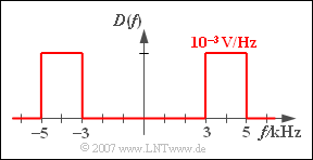
| − | '''(3)''' | + | '''(3)''' From $d(t) = x(t) - y(t)$ follows because of the linearity of the Fourier transform: $D(f) = X(f) - Y(f).$ |
| − | * | + | *The difference of the two equal high rectangular functions leads to a rectangular band-pass spectrum between $3 \,\text{kHz}$ and $5 \,\text{kHz}$. |
| − | * | + | *The (one-sided) bandwidth is thus $B_d \;\underline{= 2 \,\text{kHz}}$. In this frequency interval $D(f) = 1 \,\text{mV/Hz}$. Outside, i.e. also at $f = 0$, $D(f)\;\underline{ = 0}$ applies. |
| − | '''(4)''' | + | '''(4)''' According to the fundamental laws of the Fourier transform, the integral over the time function is equal to the spectral value at $f = 0$. It follows: : |
:$$F_x = X(f=0) = \frac{x(t=0)}{2 \cdot B_x} = 10^{-3} | :$$F_x = X(f=0) = \frac{x(t=0)}{2 \cdot B_x} = 10^{-3} | ||
| Line 121: | Line 120: | ||
:$$F_d = D(f=0) \hspace{0.15 cm}\underline{= 0}.$$ | :$$F_d = D(f=0) \hspace{0.15 cm}\underline{= 0}.$$ | ||
| − | ⇒ | + | ⇒ For each band-pass signal, the areas of the positive signal components are equal to the areas of the negative components. |
| − | |||
| − | '''(5)''' In | + | '''(5)''' In both cases, the calculation of the signal energy is easier in the frequency domain than in the time domain, because here the integration can be reduced to an area calculation of rectangles: |
:$$E_x = (10^{-3} \hspace{0.1cm}{\rm V/Hz})^2 \cdot 2 \cdot 5 | :$$E_x = (10^{-3} \hspace{0.1cm}{\rm V/Hz})^2 \cdot 2 \cdot 5 | ||
| Line 137: | Line 135: | ||
__NOEDITSECTION__ | __NOEDITSECTION__ | ||
| − | [[Category: | + | [[Category:Signal Representation: Exercises|^4.1 Differences between Low-Pass and Band-Pass^]] |
Latest revision as of 15:38, 5 May 2021
Three signal curves are sketched on the right, the first two having the following curve:
- $$x(t) = 10\hspace{0.05cm}{\rm V} \cdot {\rm si} ( \pi \cdot {t}/{T_x}) ,$$
- $$y(t) = 6\hspace{0.05cm}{\rm V} \cdot {\rm si}( \pi \cdot {t}/{T_y}) .$$
$T_x = 100 \,{\rm µ}\text{s}$ and $T_y = 166.67 \,{\rm µ}\text{s}$ indicate the first zero of $x(t)$ and $y(t)$ respectively. The signal $d(t)$ results from the difference of the two upper signals (lower graph):
- $$d(t) = x(t)-y(t) .$$
In subtask (4) the integral areas of the pulses $x(t)$ and $d(t)$ are asked for. For these holds:
- $$F_x = \int_{- \infty}^{+\infty}\hspace{-0.4cm}x(t)\hspace{0.1cm}{\rm d}t , \hspace{0.5cm}F_d = \int_{- \infty}^{+\infty}\hspace{-0.4cm}d(t)\hspace{0.1cm}{\rm d}t .$$
On the other hand, for the corresponding signal energies with Parseval's theorem:
- $$E_x = \int_{- \infty}^{+\infty}\hspace{-0.4cm}|x(t)|^2\hspace{0.1cm}{\rm d}t = \int_{- \infty}^{+\infty}\hspace{-0.4cm}|X(f)|^2\hspace{0.1cm}{\rm d}f ,$$
- $$E_d = \int_{- \infty}^{+\infty}\hspace{-0.4cm}|d(t)|^2\hspace{0.1cm}{\rm d}t = \int_{- \infty}^{+\infty}\hspace{-0.4cm}|D(f)|^2\hspace{0.1cm}{\rm d}f .$$
Hints:
- This exercise belongs to the chapter Differences and Similarities of Low-Pass and Band-Pass Signals.
- The inverse Fourier transform of a rectangular spectrum $X(f)$ leads to an $\rm si$–shaped time function $x(t)$:
- $$X(f)=\left\{ {X_0 \; \rm f\ddot{u}r\; |\it f| < \rm B, \atop {\rm 0 \;\;\; \rm sonst}}\right. \;\; \bullet\!\!-\!\!\!-\!\!\!-\!\!\circ\, \;\;x(t) = 2 \cdot X_0 \cdot B \cdot {\rm si} ( 2\pi B t) .$$
- In this task, the function $\rm si(x) = \rm sin(x)/x = \rm sinc(x/π)$ is used.
Questions
Solution
- The absolute, two-sided bandwidth $2 \cdot B_x$ is equal to the reciprocal of the first zero. It follows that:
- $$B_x = \frac{1}{2 \cdot T_x} = \frac{1}{2 \cdot 0.1 \hspace{0.1cm}{\rm ms}}\hspace{0.15 cm}\underline{ = 5 \hspace{0.1cm}{\rm kHz}}.$$
- Since the signal value at $t = 0$ is equal to the rectangular area, the constant height is given by:
- $$X(f=0) = \frac{x(t=0)}{2 B_x} = \frac{10 \hspace{0.1cm}{\rm V}}{10 \hspace{0.1cm}{\rm kHz}} \hspace{0.15 cm}\underline{= 1 \hspace{0.1cm}{\rm mV/Hz}}.$$
(2) From $T_y = 0.167 \,\text{ms}$ we get $B_y \;\underline{= 3 \,\text{kHz}}$.
- Together with $y(t = 0) = 6\,\text{V}$ this leads to the same spectral value $Y(f = 0)\; \underline{= 1\, \text{mV/Hz}}$ as in subtaske (1).
(3) From $d(t) = x(t) - y(t)$ follows because of the linearity of the Fourier transform: $D(f) = X(f) - Y(f).$
- The difference of the two equal high rectangular functions leads to a rectangular band-pass spectrum between $3 \,\text{kHz}$ and $5 \,\text{kHz}$.
- The (one-sided) bandwidth is thus $B_d \;\underline{= 2 \,\text{kHz}}$. In this frequency interval $D(f) = 1 \,\text{mV/Hz}$. Outside, i.e. also at $f = 0$, $D(f)\;\underline{ = 0}$ applies.
(4) According to the fundamental laws of the Fourier transform, the integral over the time function is equal to the spectral value at $f = 0$. It follows: :
- $$F_x = X(f=0) = \frac{x(t=0)}{2 \cdot B_x} = 10^{-3} \hspace{0.1cm}{\rm V/Hz}\hspace{0.15 cm}\underline{= 0.001 \hspace{0.1cm}{\rm Vs}},$$
- $$F_d = D(f=0) \hspace{0.15 cm}\underline{= 0}.$$
⇒ For each band-pass signal, the areas of the positive signal components are equal to the areas of the negative components.
(5) In both cases, the calculation of the signal energy is easier in the frequency domain than in the time domain, because here the integration can be reduced to an area calculation of rectangles:
- $$E_x = (10^{-3} \hspace{0.1cm}{\rm V/Hz})^2 \cdot 2 \cdot 5 \hspace{0.1cm}{\rm kHz} \hspace{0.15 cm}\underline{= 0.01 \hspace{0.1cm}{\rm V^2s}},$$
- $$E_d = (10^{-3} \hspace{0.1cm}{\rm V/Hz})^2 \cdot 2 \cdot 2 \hspace{0.1cm}{\rm kHz} \hspace{0.15 cm}\underline{= 0.004 \hspace{0.1cm}{\rm V^2s}}.$$

