Difference between revisions of "Digital Signal Transmission/Binary Symmetric Channel"
| (2 intermediate revisions by the same user not shown) | |||
| Line 48: | Line 48: | ||
*This fact is somewhat surprising at first glance: | *This fact is somewhat surprising at first glance: | ||
| − | :With $p = 0.01$, for example, the mean error distance is ${\rm E}\big[a\big] = 100$. Nevertheless, two consecutive errors $(a = 1)$ are more probable by a factor of $0.99^{99} \approx 2.7$ than the error distance $a = 100$. | + | :With $p = 0.01$, for example, the mean error distance is ${\rm E}\big[a\big] = 100$. Nevertheless, two consecutive errors $(a = 1)$ are more probable by a factor of $0.99^{99} \approx 2.7$ than the error distance $a = 100$.<br> |
*The error distance distribution is obtained by summation according to the [[Digital_Signal_Transmission/Parameters_of_Digital_Channel_Models#Error_distance_distribution|"general definition"]]: | *The error distance distribution is obtained by summation according to the [[Digital_Signal_Transmission/Parameters_of_Digital_Channel_Models#Error_distance_distribution|"general definition"]]: | ||
| Line 71: | Line 71: | ||
<br> | <br> | ||
The BSC model is the "digital equivalent" of the simplest analog model ⇒ [[Digital_Signal_Transmission/Structure_of_the_Optimal_Receiver#Some_properties_of_the_AWGN_channel|"AWGN"]] for a time-invariant digital system corresponding to the following graph. It holds | The BSC model is the "digital equivalent" of the simplest analog model ⇒ [[Digital_Signal_Transmission/Structure_of_the_Optimal_Receiver#Some_properties_of_the_AWGN_channel|"AWGN"]] for a time-invariant digital system corresponding to the following graph. It holds | ||
| − | [[File: | + | [[File:EN_Dig_T_5_2_S2b.png|right|frame|On the use of the BSC model|class=fit]] |
#The only degradation is noise. | #The only degradation is noise. | ||
#There is no distortion.<br> | #There is no distortion.<br> | ||
| Line 85: | Line 85: | ||
*threshold decision with symmetric decision threshold,<br> | *threshold decision with symmetric decision threshold,<br> | ||
| − | *no extraneous influences such as crosstalk, dial pulses, electromagnetic fields, ...<br> | + | *no extraneous interference influences such as: <br>crosstalk, dial pulses, electromagnetic fields, ...<br> |
| Line 91: | Line 91: | ||
*the application of the BSC model is often justified, | *the application of the BSC model is often justified, | ||
| − | *but not if fading influences $($ | + | *but not if fading influences $($[[Digital_Signal_Transmission/Carrier_Frequency_Systems_with_Non-Coherent_Demodulation#Rayleigh_and_Rice_Distribution|"Rayleigh or Rice"]]$)$ play a role or if echoes may occur <br>⇒ [[Mobile_Communications/Multi-Path_Reception_in_Mobile_Communications|"multi-path reception"]].<br> |
Latest revision as of 16:23, 6 September 2022
Contents
Binary Symmetric Channel – Model and Error Correlation Function
The left graph shows the BSC model, the simplest model of a digital transmission system.
The name stands for "Binary Symmetric Channel" and states that this model can only be used for binary systems with symmetrical falsification properties.
Further applies:
- The BSC model is suitable for the study and generation of an error sequence with statistically independent errors.
- Such a channel is also called "memory-free" and unlike the "burst error channel models" only a single channel state exists.
- The two symbols $($for example $\rm L$ and $\rm H)$ are each falsified with the same probability $p$, so that the mean error probability $p_{\rm M} = p$ is also independent of the symbol probabilities $p_{\rm L}$ and $p_{\rm H}$.
The right graph shows the "error correlation function" $\rm (ECF)$ of the BSC model:
- \[\varphi_{e}(k) = {\rm E}\big[e_{\nu} \cdot e_{\nu + k}\big] = \left\{ \begin{array}{c} p \\ p^2 \end{array} \right.\quad \begin{array}{*{1}c} f{\rm or }\hspace{0.25cm}k = 0 \hspace{0.05cm}, \\ f{\rm or }\hspace{0.25cm} k > 0 \hspace{0.05cm}.\\ \end{array}\]
$\text{Conclusion:}$
- In the BSC model, the final ECF value $($square of the mean error probability$)$, which in other models is valid only for $k \to \infty$, is reached exactly at $k = 1$ and then remains constant.
- The BSC model belongs to the class of "renewal channel models". In a renewal channel model, the error distances are statistically independent of each other and the error correlation function can be calculated iteratively in a simple way:
- \[\varphi_{e}(k) = \sum_{\kappa = 1}^{k} {\rm Pr}(a = \kappa) \cdot \varphi_{e}(k - \kappa) \hspace{0.05cm}.\]
Binary Symmetric Channel – Error Distance Distribution
We now consider the "error distance distribution" $\rm (EDD)$. The probability for the error distance $a=k$ is obtained from the condition of $k-1$ error-free symbols and one transmission error at time $\nu +k$, assuming that the last error occurred at time $\nu$. One obtains:
- \[{\rm Pr}(a = k) = (1-p)^{k-1}\cdot p \hspace{0.05cm}.\]
It follows:
- The error distance $a = 1$ always occurs in the BSC model with the greatest probability, and this for any value of $p$.
- This fact is somewhat surprising at first glance:
- With $p = 0.01$, for example, the mean error distance is ${\rm E}\big[a\big] = 100$. Nevertheless, two consecutive errors $(a = 1)$ are more probable by a factor of $0.99^{99} \approx 2.7$ than the error distance $a = 100$.
- The error distance distribution is obtained by summation according to the "general definition":
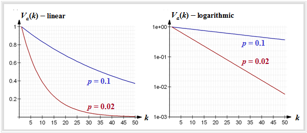
- \[V_a(k) = {\rm Pr}(a \ge k) = 1 - \sum_{\kappa = 1}^{k} (1-p)^{\kappa-1}\cdot p = (1-p)^{k-1}\hspace{0.05cm}.\]
$\text{Example 1:}$ The left graph shows $V_a(k)$ in linear representation for
- $p = 0.1$ (blue curve), and
- $p = 0.02$ (red curve).
⇒ The decrease is exponential with increasing $k$ and is steeper the smaller $p$ is.
⇒ The right graph shows the logarithmic representation. Here the drop is linear according to
- \[{\rm lg} \hspace{0.15cm}V_a(k) = (k - 1) \cdot {\rm lg} \hspace{0.15cm}(1-p)\hspace{0.05cm}.\]
Applications of the BSC model
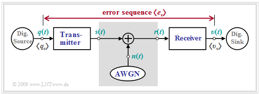
The BSC model is the "digital equivalent" of the simplest analog model ⇒ "AWGN" for a time-invariant digital system corresponding to the following graph. It holds
- The only degradation is noise.
- There is no distortion.
To use the BSC model, the digital system must meet the following requirements:
- Redundancy-free binary encoding ⇒ no channel encoding and decoding,
- noise according to the AWGN model ⇒ additive, white, Gaussian distributed,
- no $($linear & non-linear$)$ distortions due to transmitter / receiver components,
- threshold decision with symmetric decision threshold,
- no extraneous interference influences such as:
crosstalk, dial pulses, electromagnetic fields, ...
For a "radio system" with a direct line-of-sight between transmitter and receiver,
- the application of the BSC model is often justified,
- but not if fading influences $($"Rayleigh or Rice"$)$ play a role or if echoes may occur
⇒ "multi-path reception".
⇒ In contrast, according to network operators, statistically independent errors tend to be the exception in the case of "wireline transmission"
(e.g. "DSL", but also optical transmission$)$.
⇒ If errors occur during data transmission via the telephone network, they are usually clustered. In this case, we speak of so-called "burst errors", which will be discussed in the next chapter.
Exercises for the chapter
Exercise 5.3: AWGN and BSC Model
Exercise 5.3Z: Analysis of the BSC Model
Exercise 5.4: Is the BSC Model Renewing?
Exercise 5.5: Error Sequence and Error Distance Sequence


