Aufgaben:Exercise 1.7Z: Overall Systems Analysis

• Return to book

System with Gaussian low-passe filters and non-linear characteristic curve

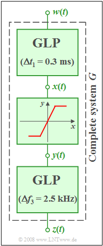
An overall system  $G$  with input $w(t)$  and output  $z(t)$  consists of three components:

• The first component is a Gaussian low-pass filter with impulse response

$$h_1(t) = \frac{1}{\Delta t_1} \cdot {\rm e}^{-\pi\hspace{0.05cm}\cdot \hspace{0.05cm} (t/\Delta t_1)^2}, \hspace{0.5cm} \Delta t_1= {0.3\,\rm ms}.$$

• This is then followed by a non-linearity with the characteristic curve

$$y(t) = \left\{ \begin{array}{c} +{8\,\rm V} \\ 2 \cdot x(t) \\ {-8\,\rm V} \\ \end{array} \right.\quad \quad \begin{array}{*{10}c} {\rm{f\ddot{u}r}} \\ {\rm{f\ddot{u}r}} \\ {\rm{f\ddot{u}r}} \\ \end{array}\begin{array}{*{20}c} {x(t) \ge +{4\,\rm V}}, \\ {{-4\,\rm V} < x(t) < +{4\,\rm V}}, \\ {x(t)\le {-4\,\rm V}}. \\ \end{array}$$

⇒   The input signal  $x(t)$  of the non-linearity is amplified by the factor  $2$  and – if necessary – limited to the range  $±8 \ \rm V$ .

• At the end of the chain there is again a Gaussian low-pass filter given by its frequency response:

$$H_3(f) = {\rm e}^{-\pi\hspace{0.05cm}\cdot \hspace{0.05cm}(f/\Delta f_3)^2}, \hspace{0.5cm} \Delta f_3= {2.5\,\rm kHz}.$$

Let the input signal $w(t)$  of the overall system be a Gaussian pulse with amplitude  $5 \ \rm V$  and variable (equivalent) duration  $T$:

$$w(t) = {5\,\rm V}\cdot {\rm e}^{-\pi\hspace{0.05cm}\cdot \hspace{0.05cm}(t/T)^2}.$$

What needs to be investigated is the range in which the equivalent impulse duration  $T$  of this Gaussian pulse can vary such that the overall system can be entirely described by the frequency response

$$H_{\rm G}(f) = K \cdot {\rm e}^{-\pi\hspace{0.05cm}\cdot \hspace{0.05cm}(f/\Delta f_{\rm G})^2}.$$

Here, the subscript "G" in frequency response and bandwidth stands for "Gesamtsystem" (German for "overall system").

Please note:

• The exercise belongs to the chapter   Some Low-Pass Functions in Systems Theory.
• Reference is made especially to the page  Gaussian low-pass filter.

Questions

1

What conditions must be satisfied for the overall system to be describable by a single frequency response?

	There is a linear relationship between  $w(t)$  and  $z(t)$.
	$H_3(f)$  must be more narrow-band than  $H_1(f)$.
	The signal  $x(t)$  must not be greater in magnitude than  $4 \ \rm V$.

2

Compute the maximum value for the equivalent impulse duration  $T$ so that the conditions given in  (1)  are satisfiable.

$T_{\rm max} \ = \ $ $\ \rm ms$

3

Specify the parameters of the overall frequency response  $H_{\rm G}(f)$ .

$K \ = \ $

$\Delta f_{\rm G} = \ $ $\ \rm kHz$

Solution

Solution

(1)  Answers 1 and 3 are correct:

• The first statement is correct:   Only for a linear system a frequency response can be specified.
• For this to be possible here nonlinearity must not play a role.
• That is, it must be ensured that  $|x(t)|$  is not greater than  $4 \ \rm V$ .
• In contrast to this, the second statement is not true:   The bandwidth of  $H_3(f)$  does not affect whether the non-linearity can be eliminated or not.

(2)  The first Gaussian low-pass filter is described in the frequency domain as follows:

$$X(f) = W(f) \cdot H_1(f) = {5\,\rm V}\cdot T \cdot {\rm e}^{-\pi(f \cdot T)^2} \cdot {\rm e}^{-\pi(f/\Delta f_1)^2} = {5\,\rm V}\cdot T \cdot {\rm e}^{-\pi f^2 (T^2 + \Delta t_1^2)}= {5\,\rm V}\cdot T \cdot {\rm e}^{-\pi(f/\Delta f_x)^2}.$$

• Here,   $Δf_x$  denotes the equivalent bandwidth of  $X(f)$.
• The signal value at  $t = 0$  is equal to the spectral area and at the same time to the maximum value of the signal:
• This should not exceed $4 \ \rm V$:

$$x_{\rm max} = x(t =0) = {5\,\rm V}\cdot T \cdot \Delta f_x \le {4\,\rm V}.$$

• From this it follows by comparison of coefficients:

$$\frac{1}{T \cdot \Delta f_x} > \frac{5}{4}\hspace{0.1cm} \Rightarrow \hspace{0.1cm} \frac{1}{T^2 \cdot \Delta f_x^2} > \frac{25}{16} \Rightarrow \hspace{0.3cm}\frac{T^2 + \Delta t_1^2}{T^2} > \frac{25}{16}$$

$$ \Rightarrow \hspace{0.1cm}\frac{ \Delta t_1^2}{T^2} > \frac{9}{16}\hspace{0.3cm}\Rightarrow \hspace{0.5cm}\frac{T^2}{ \Delta t_1^2} \le \frac{16}{9}\hspace{0.3cm}\Rightarrow \hspace{0.3cm} T \le \frac{4}{3} \cdot \Delta t_1 \hspace{0.15cm}\underline{= {0.4\,\rm ms}}.$$

• The control calculation yields:

$$\Delta t_x = \sqrt{T^2 + \Delta t_1^2} = \sqrt{({0.4\,\rm ms})^2 + ({0.3\,\rm ms})^2} = {0.5\,\rm ms} \hspace{0.3cm}\Rightarrow \hspace{0.3cm}\Delta f_x = {1}/{\Delta t_x}= {2\,\rm kHz}$$

$$\Rightarrow \hspace{0.3cm} x(t=0) = {5\,\rm V}\cdot T \cdot \Delta f_x = {5\,\rm V}\cdot {0.4\,\rm ms} \cdot {2\,\rm kHz} = {4\,\rm V}.$$

(3)  The Gaussian low-pass filters satisfy the condition  $H_1(f = 0) = H_3(f = 0) = 1$.

• Taking into account the gain of the second block in the linear domain the following is thus obtained for the total gain:

$$\underline{K \ = \ 2}.$$

• For the equivalent impulse duration of the overall system it holds that:

$$\Delta t_{\rm G} = \sqrt{\Delta t_1^2 + \frac{1}{\Delta f_3^2}} = \sqrt{({0.3\,\rm ms})^2 + \left( \frac{1}{{2.5\,\rm kHz}}\right)^2}={0.5\,\rm ms} \; \; \Rightarrow \; \; \Delta f_{\rm G} = {1}/{\Delta t_{\rm G}} \hspace{0.15cm}\underline{= {2\,\rm kHz}}.$$