Aufgaben:Exercise 3.6Z: Two Imaginary Poles

• Return to book

Two imaginary poles and one zero

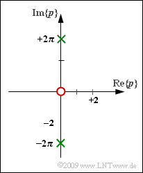
In this exercise, we consider a causal signal  $x(t)$  with the Laplace transform

$$X_{\rm L}(p) = \frac { p} { p^2 + 4 \pi^2}= \frac { p} { (p-{\rm j} \cdot 2\pi)(p+{\rm j} \cdot 2\pi)} \hspace{0.05cm}$$

corresponding to the graph  (one red zero and two green poles).

In contrast, the signal  $y(t)$  has the Laplace spectral function

$$Y_{\rm L}(p) = \frac { 1} { p^2 + 4 \pi^2} \hspace{0.05cm}.$$

Thus, the red zero does not belong to  $Y_{\rm L}(p)$.

Finally, the signal  $z(t)$  with the Laplace tansform

$$Z_{\rm L}(p) = \frac { p} { (p-{\rm j} \cdot \beta)(p+{\rm j} \cdot \beta)} \hspace{0.05cm}$$

is considered, in particular the limiting case for  $\beta → 0$.

Please note:

• The exercise belongs to the chapter  Inverse Laplace Transform.
• The frequency variable  $p$  is normalized such that time  $t$  is in microseconds after applying the residue theorem.
• A result  $t = 1$  is thus to be interpreted as  $t = T$  with  $T = 1 \ \rm µ s$ .
• The  residue theorem  is as follows using the example of the function  $X_{\rm L}(p)$  with two simple poles at  $\pm {\rm j} \cdot \beta$:

$$x(t) = X_{\rm L}(p) \cdot (p - {\rm j} \cdot \beta) \cdot {\rm e}^{\hspace{0.03cm}p\hspace{0.05cm} \cdot \hspace{0.05cm}t} \Bigg |_{\hspace{0.1cm} p\hspace{0.05cm}=\hspace{0.05cm}{\rm j \hspace{0.05cm} \cdot\hspace{0.05cm} \it \beta}}+X_{\rm L}(p) \cdot (p + {\rm j} \cdot \beta) \cdot {\rm e}^{\hspace{0.03cm}p \hspace{0.05cm} \cdot\hspace{0.05cm}t} \Bigg |_{\hspace{0.1cm} p\hspace{0.05cm}=\hspace{0.05cm}{-\rm j \hspace{0.05cm} \cdot\hspace{0.05cm} \it \beta}} \hspace{0.05cm}.$$

Questions

1

Compute the signal  $x(t)$. Which of the following statements are correct?

	$x(t)$  is a causal cosine signal.
	$x(t)$  is a causal sinusoidal signal.
	The amplitude of  $x(t)$  is  $1$.
	The period of $x(t)$ is  $T = 1 \ \rm µ s$.

2

Compute the signal  $y(t)$. Which of the following statements are correct?

	$y(t)$  is a causal cosine signal.
	$y(t)$  is a causal sinusoidal signal.
	The amplitude of  $y(t)$  is  $1$.
	The period of  $y(t)$  is  $T = 1 \ \rm µ s$.

3

Which statements are true for the signal  $z(t)$ ?

	For  $\beta > 0$,   $z(t)$  is cosine-shaped.
	For  $\beta > 0$,   $z(t)$  is sinusoidal.
	The limiting case  $\beta → 0$  results in the step function  $\gamma(t)$.

Solution

Solution

(1)  The suggested solutions 1, 3 and 4 are correct:

• The following is obtained for signal  $x(t)$  for positive times by applying the residue theorem:

$$x_1(t)\hspace{0.25cm} = \hspace{0.2cm} {\rm Res} \bigg |_{p \hspace{0.05cm}= \hspace{0.05cm}p_{{\rm x}1}} \hspace{0.7cm}\{X_{\rm L}(p)\cdot {\rm e}^{\hspace{0.05cm}p \hspace{0.05cm}\cdot \hspace{0.05cm}t}\}= \frac {p} { p+{\rm j} \cdot 2\pi}\cdot {\rm e}^{\hspace{0.05cm}p \hspace{0.05cm}\cdot \hspace{0.05cm}t} \bigg |_{p \hspace{0.05cm}= \hspace{0.05cm}{\rm j} \hspace{0.05cm}\cdot \hspace{0.05cm}2\pi}= \frac{1}{2} \cdot {\rm e}^{\hspace{0.05cm}{\rm j} \hspace{0.05cm} \cdot \hspace{0.05cm}2\pi t}\hspace{0.05cm} ,$$

$$x_2(t)\hspace{0.25cm} = \hspace{0.2cm} {\rm Res} \bigg |_{p \hspace{0.05cm}= \hspace{0.05cm}p_{{\rm x}2}} \hspace{0.7cm}\{X_{\rm L}(p)\cdot {\rm e}^{\hspace{0.05cm}p \hspace{0.05cm}\cdot \hspace{0.05cm} t}\}= \frac {p} { p-{\rm j} \cdot 2\pi}\cdot {\rm e}^{\hspace{0.05cm}p \hspace{0.05cm}\cdot \hspace{0.05cm}t} \bigg |_{p \hspace{0.05cm}= -{\rm j} \hspace{0.05cm}\cdot \hspace{0.05cm}2\pi}= \frac{1}{2} \cdot {\rm e}^{-{\rm j} \hspace{0.05cm} \cdot \hspace{0.05cm}2\pi t} \hspace{0.05cm} .$$

$$\Rightarrow \hspace{0.3cm} x(t) = x_1(t) + x_2(t) = {1}/{2} \cdot \left [ {\rm e}^{\hspace{0.05cm}{\rm j} \hspace{0.05cm} \cdot \hspace{0.05cm}2\pi t}+{\rm e}^{-{\rm j} \hspace{0.05cm} \cdot \hspace{0.05cm}2\pi t}\right ] = \cos(2\pi t) \hspace{0.05cm} .$$

(2)  The suggested solutions 2 and 4 are correct:

• In principle, this subtask could be solved in the same way as subtask  (1).
• However, the integration theorem can also be used.
• This says among other things that multiplication by  $1/p$  in the spectral domain corresponds to integration in the time domain:

$$Y_{\rm L}(p) = {1}/{p} \cdot X_{\rm L}(p) \hspace{0.3cm} \Rightarrow \hspace{0.3cm} t \ge 0:\quad y(t) = \int_{-\infty}^t \cos(2\pi \tau)\,\,{\rm d}\tau = {1}/({2\pi}) \cdot \sin(2\pi t) \hspace{0.05cm} .$$

Please note:     The causal cosine signal  $x(t)$  and the causal sine signal  $y(t)$  are shown on the information page of  Exercise 3.6  as  $c_{\rm K}(t)$  and  $s_{\rm K}(t)$,  respectively.

(3)  The suggested solutions 1 and 3 are correct:

• A comparison with the computation of  $x(t)$  shows that  $z(t) = \cos (\beta \cdot t)$  holds for  $t \ge 0$  and  $z(t) = 0$  for  $t < 0$ .
• The limit process for  $\beta → 0$  thus results in the step function  $\gamma(t)$.
• The same result is obtained by consideration in the spectral domain:

$$Z_{\rm L}(p) = \lim_{\beta \hspace{0.05cm} \rightarrow \hspace{0.05cm} 0}\hspace{0.1cm}\frac{p}{p^2 + \beta^2} = {1}/{p} \hspace{0.3cm} \Rightarrow \hspace{0.3cm} z(t) = \gamma(t) \hspace{0.05cm} .$$