Theory of Stochastic Signals/Stochastic System Theory: Difference between revisions
No edit summary |
No edit summary |
||
| Line 1: | Line 1: | ||
{{Header | {{Header | ||
|Untermenü= | |Untermenü=Filtering of Stochastic Signals | ||
|Vorherige Seite= Verallgemeinerung auf N-dimensionale Zufallsgrößen | |Vorherige Seite= Verallgemeinerung auf N-dimensionale Zufallsgrößen | ||
|Nächste Seite=Digitale Filter | |Nächste Seite=Digitale Filter | ||
}} | }} | ||
== # | == # OVERVIEW OF THE FIFTH MAIN CHAPTER # == | ||
<br> | <br> | ||
his chapter describes the influence of a filter on the auto-correlation function (ACF) and the power density spectrum (PDS) of stochastic signals. | |||
In detail, it covers: | |||
* | *the calculation of ACF and PDS at the filter output (''Stochastic System Theory'' ), | ||
* | *the structure and representation of ''digital filters'' (non-recursive and recursive), | ||
* | *the ''dimensioning'' of filter coefficients for a given ACF, | ||
* | *the meaning of the 'matched filter'' communication systems (SNR maximization), | ||
* | *the properties of the ''Wiener-Kolmogorow filter'' for signal reconstruction. | ||
| Line 22: | Line 22: | ||
== | ==Problem== | ||
<br> | <br> | ||
[[File:EN_Sto_T_5_1_S1.png |right| 300px|frame| | [[File:EN_Sto_T_5_1_S1.png |right| 300px|frame|Filter influence on spectrum and power density spectrum (PDS)]] | ||
As in the book [[Linear and Time-Invariant Systems]], we consider the setup sketched on the right, where the system | |||
* | *characterized both by the impulse response $h(t)$ | ||
* | *as well as by its frequency response $H(f)$ | ||
is described unambiguously. The relationship between these descriptive quantities in the time and frequency domain is given by the [[Signal_Representation/Fourier_Transform_and_its_Inverse#Properties_of_aperiodic_signals|Fourier transformation]]. | |||
<br clear=all> | <br clear=all> | ||
If we apply the signal $x(t)$ to the input and denote the output signal by $y(t)$, classical system theory provides the following statements: | |||
* | *The output signal $y(t)$ results from the [[Signal_Representation/The_Convolution_Theorem_and_Operation|convolution]] between the input signal $x(t)$ and the impulse response $h(t)$. The following equation is equally valid for deterministic and stochastic signals: | ||
:$$y(t) = x(t) \ast h(t) = \int_{-\infty}^{+\infty} x(\tau)\cdot h ( t - \tau) \,\,{\rm d}\tau.$$ | :$$y(t) = x(t) \ast h(t) = \int_{-\infty}^{+\infty} x(\tau)\cdot h ( t - \tau) \,\,{\rm d}\tau.$$ | ||
* | *For deterministic signals, one usually takes a roundabout route using the spectral functions. The spectrum $X(f)$ is the Fourier transform of $x(t)$. The multiplication with the frequency response $H(f)$ leads to the output spectrum $Y(f)$. From this, the signal $y(t)$ can be obtained by Fourier inverse transformation. | ||
* | *In the case of stochastic signals this procedure fails, because then the time functions $x(t)$ and $y(t)$ are not predictable for all times from $–∞$ to $+∞$ and thus the corresponding amplitude spectra $X(f)$ and $Y(f)$ do not exist at all. | ||
*In | *In this case, we have to switch to the [[Theory_of_Stochastic_Signals/Leistungsdichtespektrum_(LDS)|power density spectra]] defined in the last chapter. | ||
== | ==Amplitude and power density spectrum== | ||
<br> | <br> | ||
We consider an ergodic random process $\{x(t)\}$, whose auto-correlation function $φ_x(τ)$ is assumed to be known. The power density spectrum ${\it Φ}_x(f)$ is then also uniquely determined via the Fourier transform and the following statements hold: | |||
:[[File:P_ID467__Sto_T_5_1_S2_neu.png|right| |frame| | :[[File:P_ID467__Sto_T_5_1_S2_neu.png|right| |frame| For the ACF and PDS calculation of a random signal]] | ||
* | *The power density spectrum ${\it Φ}_x(f)$ can be given – as well as the auto-correlation function $φ_x(τ)$ – for each individual pattern function of the stationary and ergodic random process $\{x(t)\}$, even if the specific course of $x(t)$ is explicitly unknown. | ||
* | *The [[Signal_Representation/Fourier_Transform_and_its_Inverse#The_first_Fourier_integral|amplitude spectrum]] $X(f)$, on the other hand, is undefined because if the spectral function $X(f)$ is known, the entire time function $x(t)$ from $–∞$ to $+∞$ would also have to be known via the Fourier inverse transform, which clearly cannot be the case for a stochastic signal. | ||
* | *If a time section of the finite time duration $T_{\rm M}$ is known according to the sketch on the left, the Fourier transform can of course be applied to it again. | ||
<br clear=all> | <br clear=all> | ||
{{BlaueBox|TEXT= | {{BlaueBox|TEXT= | ||
$\text{ | $\text{Theorem:}$ The following relationship exists between the power density spectrum ${\it Φ}_x(f)$ of the infinite time random signal $x(t)$ and the amplitude spectrum $X_{\rm T}(f)$ of the finite time section $x_{\rm T}(t)$: | ||
:$${ {\it \Phi}_x(f)} = \lim_{T_{\rm M}\to\infty}\hspace{0.2cm} | :$${ {\it \Phi}_x(f)} = \lim_{T_{\rm M}\to\infty}\hspace{0.2cm} | ||
\frac{1}{ T_{\rm M} }\cdot \vert X_{\rm T}(f)\vert ^2.$$}} | \frac{1}{ T_{\rm M} }\cdot \vert X_{\rm T}(f)\vert ^2.$$}} | ||
| Line 55: | Line 55: | ||
{{BlaueBox|TEXT= | {{BlaueBox|TEXT= | ||
$\text{ | $\text{Proof:}$ Previously, the | ||
[[Theory_of_Stochastic_Signals/ | [[Theory_of_Stochastic_Signals/Auto-Correlation_Function_(ACF)|auto-correlation function]] of an ergodic process with the sample function $x(t)$ was given as follows: | ||
:$${ {\it \varphi}_x(\tau)} = \lim_{T_{\rm M}\to\infty}\hspace{0.2cm} | :$${ {\it \varphi}_x(\tau)} = \lim_{T_{\rm M}\to\infty}\hspace{0.2cm} | ||
\frac{1}{ T_{\rm M} }\cdot\int^{+T_{\rm M}/2}_{-T_{\rm | \frac{1}{ T_{\rm M} }\cdot\int^{+T_{\rm M}/2}_{-T_{\rm | ||
M}/2}x(t)\cdot x(t + \tau)\hspace{0.1cm} \rm d \it t.$$ | M}/2}x(t)\cdot x(t + \tau)\hspace{0.1cm} \rm d \it t.$$ | ||
* | *It is permissible to replace the function $x(t)$, which is unbounded in time, by the function $x_{\rm T}(t)$, which is bounded on the time range $-T_{\rm M}/2$ to $+T_{\rm M}/2$. $x_{\rm T}(t)$ corresponds to the spectrum $X_{\rm T}(f)$, and by applying the [[Signal_Representation/Fourier_Transform_and_its_Inverse#The_first_Fourier_integral|first Fourier integral]] and the [[Signal_Representation/Fourier_Transform_Theorems#Shifting_Theorem|shifting theorem]]: | ||
:$${ {\it \varphi}_x(\tau)} = \lim_{T_{\rm M}\to\infty}\hspace{0.2cm} | :$${ {\it \varphi}_x(\tau)} = \lim_{T_{\rm M}\to\infty}\hspace{0.2cm} | ||
\frac{1}{ T_{\rm M} }\cdot \int^{+T_{\rm M}/2}_{-T_{\rm | \frac{1}{ T_{\rm M} }\cdot \int^{+T_{\rm M}/2}_{-T_{\rm | ||
| Line 66: | Line 66: | ||
T}(f)\cdot {\rm e}^{ {\rm j}2 \pi f ( t + \tau) } \hspace{0.1cm} | T}(f)\cdot {\rm e}^{ {\rm j}2 \pi f ( t + \tau) } \hspace{0.1cm} | ||
\rm d \it f \hspace{0.1cm} \rm d \it t.$$ | \rm d \it f \hspace{0.1cm} \rm d \it t.$$ | ||
* | *After splitting the exponent and swapping the time and frequency integrals, we get: | ||
:$${ {\it \varphi}_x(\tau)} = \lim_{T_{\rm M}\to\infty}\hspace{0.2cm} | :$${ {\it \varphi}_x(\tau)} = \lim_{T_{\rm M}\to\infty}\hspace{0.2cm} | ||
\frac{1}{ T_{\rm M} }\cdot \int^{+\infty}_{-\infty}X_{\rm | \frac{1}{ T_{\rm M} }\cdot \int^{+\infty}_{-\infty}X_{\rm | ||
| Line 72: | Line 72: | ||
T}(t)\cdot {\rm e}^{ {\rm j}2 \pi f t } \hspace{0.1cm} \rm d \it | T}(t)\cdot {\rm e}^{ {\rm j}2 \pi f t } \hspace{0.1cm} \rm d \it | ||
t \right] \cdot {\rm e}^{ {\rm j}2 \pi f \tau} \hspace{0.1cm} \rm d \it f.$$ | t \right] \cdot {\rm e}^{ {\rm j}2 \pi f \tau} \hspace{0.1cm} \rm d \it f.$$ | ||
* | *The inner integral describes the conjugate-complex spectrum $X_{\rm T}^{\star}(f)$. It further follows that: | ||
:$${ {\it \varphi}_x(\tau)} = \lim_{T_{\rm M}\to\infty}\hspace{0.2cm} | :$${ {\it \varphi}_x(\tau)} = \lim_{T_{\rm M}\to\infty}\hspace{0.2cm} | ||
\frac{1}{ T_{\rm M} }\cdot \int^{+\infty}_{-\infty}\vert X_{\rm | \frac{1}{ T_{\rm M} }\cdot \int^{+\infty}_{-\infty}\vert X_{\rm | ||
T}(f)\vert^2 \cdot {\rm e}^{ {\rm j}2 \pi f \tau} \hspace{0.1cm} \rm d | T}(f)\vert^2 \cdot {\rm e}^{ {\rm j}2 \pi f \tau} \hspace{0.1cm} \rm d | ||
\it f.$$ | \it f.$$ | ||
* | *A comparison with [https://en.wikipedia.org/wiki/Norbert_Wiener Wiener] and [https://en.wikipedia.org/wiki/Aleksandr_Khinchin Chintchin's] theorem which is always valid in ergodicity, | ||
:$${ {\it \varphi}_x(\tau)} = \int^{+\infty}_{-\infty}{\it \Phi}_x(f) | :$${ {\it \varphi}_x(\tau)} = \int^{+\infty}_{-\infty}{\it \Phi}_x(f) | ||
\cdot {\rm e}^{ {\rm j}2 \pi f \tau} \hspace{0.1cm} \rm d \it f ,$$ | \cdot {\rm e}^{ {\rm j}2 \pi f \tau} \hspace{0.1cm} \rm d \it f ,$$ | ||
: | :shows the validity of the above relation: | ||
:$${ {\it \Phi}_x(f)} = \lim_{T_{\rm M}\to\infty}\hspace{0.2cm} | :$${ {\it \Phi}_x(f)} = \lim_{T_{\rm M}\to\infty}\hspace{0.2cm} | ||
\frac{1}{ T_{\rm M} }\cdot \vert X_{\rm T}(f)\vert^2.$$ | \frac{1}{ T_{\rm M} }\cdot \vert X_{\rm T}(f)\vert^2.$$ | ||
<div align="right">'''q.e.d.'''</div>}} | <div align="right">'''q.e.d.'''</div>}} | ||
== | ==Power density spectrum of the filter output signal== | ||
<br> | <br> | ||
Combining the statements made in the last two sections, we arrive at the following important result: | |||
{{BlaueBox|TEXT= | {{BlaueBox|TEXT= | ||
$\text{ | $\text{Theorem:}$ The power density spectrum (PDS) at the output of a linear time-invariant system with frequency response $H(f)$ is obtained as the product of the input PDS ${\it Φ}_x(f)$ and the "power transfer function" $\vert H(f)\vert ^2$. | ||
:$${ {\it \Phi}_y(f)} = { {\it \Phi}_x(f)} \cdot \vert H(f)\vert ^2.$$}} | :$${ {\it \Phi}_y(f)} = { {\it \Phi}_x(f)} \cdot \vert H(f)\vert ^2.$$}} | ||
{{BlaueBox|TEXT= | {{BlaueBox|TEXT= | ||
$\text{ | $\text{Proof:}$ Starting from the three relations already derived before: | ||
:$${ {\it \Phi}_x(f)} =\hspace{-0.1cm} \lim_{T_{\rm M}\to\infty}\hspace{0.01cm} | :$${ {\it \Phi}_x(f)} =\hspace{-0.1cm} \lim_{T_{\rm M}\to\infty}\hspace{0.01cm} | ||
\frac{1}{ T_{\rm M} }\hspace{-0.05cm}\cdot\hspace{-0.05cm} \vert X_{\rm T}(f)\vert^2, \hspace{0.5cm} | \frac{1}{ T_{\rm M} }\hspace{-0.05cm}\cdot\hspace{-0.05cm} \vert X_{\rm T}(f)\vert^2, \hspace{0.5cm} | ||
| Line 101: | Line 101: | ||
\frac{1}{ T_{\rm M} }\hspace{-0.05cm}\cdot\hspace{-0.05cm}\vert Y_{\rm T}(f)\vert^2, \hspace{0.5cm} | \frac{1}{ T_{\rm M} }\hspace{-0.05cm}\cdot\hspace{-0.05cm}\vert Y_{\rm T}(f)\vert^2, \hspace{0.5cm} | ||
Y_{\rm T}(f) = X_{\rm T}(f) \hspace{-0.05cm}\cdot\hspace{-0.05cm} H(f).$$ | Y_{\rm T}(f) = X_{\rm T}(f) \hspace{-0.05cm}\cdot\hspace{-0.05cm} H(f).$$ | ||
Substituting these equations into each other, we get the above result. | |||
<div align="right">'''q.e.d.'''</div>}} | <div align="right">'''q.e.d.'''</div>}} | ||
The following example illustrates the relationship with white noise. | |||
[[File:P_ID468__Sto_T_5_1_S3_neu.png |right|frame| | [[File:P_ID468__Sto_T_5_1_S3_neu.png |right|frame| Filter influence in the frequency domain]] | ||
{{GraueBox|TEXT= | {{GraueBox|TEXT= | ||
$\text{ | $\text{Example 1:}$ | ||
At the input of a Gaussian low-pass filter with the frequency response | |||
:$$H(f) = {\rm e}^{- \pi \hspace{0.03cm}\cdot \hspace{0.03cm}(f/\Delta f)^2}$$ | :$$H(f) = {\rm e}^{- \pi \hspace{0.03cm}\cdot \hspace{0.03cm}(f/\Delta f)^2}$$ | ||
white noise $x(t)$ with noise power density ${ {\it \Phi}_x(f)} =N_0/2$ is present ⇒ two-sided representation. Then, the following holds for the power density spectrum of the output signal: | |||
:$${ {\it \Phi}_y(f)} = \frac {N_0}{2} \cdot {\rm e}^{- 2 \pi \hspace{0.03cm}\cdot \hspace{0.03cm}(f/\Delta | :$${ {\it \Phi}_y(f)} = \frac {N_0}{2} \cdot {\rm e}^{- 2 \pi \hspace{0.03cm}\cdot \hspace{0.03cm}(f/\Delta | ||
f)^2}.$$ | f)^2}.$$ | ||
The diagram shows the signals and power density spectra at the filter input and output. | |||
'' | ''Notes:'' | ||
# | # The signal $x(t)$ – strictly speaking – cannot be plotted at all, since it has an infinite power ⇒ integral over ${\it Φ}_x(f)$ from $-\infty$ to $+\infty$. | ||
# | # The output signal $y(t)$ has a lower frequency than $x(t)$ and a finite power corresponding to the integral over ${\it Φ}_y(f)$. | ||
# | # In one-sided representation, (only) for $f>0$ would hold: ${ {\it \Phi}_x(f)} =N_0$. he statements (1) and (2) would also apply here in the same way.}} | ||
== | ==The auto-correlation function of the filter output signal== | ||
<br> | <br> | ||
The calculated power density spectrum (PDS) can also be written as follows: | |||
:$${{\it \Phi}_y(f)} = {{\it \Phi}_x(f)} \cdot H(f) \cdot H^{\star}(f)$$ | :$${{\it \Phi}_y(f)} = {{\it \Phi}_x(f)} \cdot H(f) \cdot H^{\star}(f)$$ | ||
{{BlaueBox|TEXT= | {{BlaueBox|TEXT= | ||
$\text{ | $\text{Theorem:}$ The corresponding auto-correlation function (ACF) is then obtained according to the [[Signal_Representation/Fourier_Transform_Laws|regularities of the Fourier transform]] and by applying the [[Signal_Representation/The_Convolution_Theorem_and_Operation#Convolution_in_the_time_domain|convolution theorem]]: | ||
:$${ {\it \varphi}_y(\tau)} = { {\it \varphi}_x(\tau)} \ast h(\tau)\ast h(- | :$${ {\it \varphi}_y(\tau)} = { {\it \varphi}_x(\tau)} \ast h(\tau)\ast h(- | ||
\tau).$$}} | \tau).$$}} | ||
In the transition from the spectral to the time domain, note: | |||
* | * The Fourier retransforms are to be inserted in each case, namely | ||
:$${{\it \varphi}_y(\tau)} \circ\hspace{0.05cm}\!\!\!-\!\!\!-\!\!\!-\!\!\bullet\,{{\it \Phi}_y(f)}, \hspace{0.5cm}{{\it \varphi}_x(\tau)} \circ\hspace{0.05cm}\!\!\!-\!\!\!-\!\!\!-\!\!\!\bullet\,{{\it \Phi}_x(f)}, \hspace{0.5cm}{h(\tau)} \circ\hspace{0.05cm}\!\!\!-\!\!\!-\!\!\!-\!\!\bullet\,{H(f)}, \hspace{0.5cm}{h(-\tau)} \circ\hspace{0.05cm}\!\!\!-\!\!\!-\!\!\!-\!\!\!\bullet\,{H^{\star}(f)}$$ | :$${{\it \varphi}_y(\tau)} \circ\hspace{0.05cm}\!\!\!-\!\!\!-\!\!\!-\!\!\bullet\,{{\it \Phi}_y(f)}, \hspace{0.5cm}{{\it \varphi}_x(\tau)} \circ\hspace{0.05cm}\!\!\!-\!\!\!-\!\!\!-\!\!\!\bullet\,{{\it \Phi}_x(f)}, \hspace{0.5cm}{h(\tau)} \circ\hspace{0.05cm}\!\!\!-\!\!\!-\!\!\!-\!\!\bullet\,{H(f)}, \hspace{0.5cm}{h(-\tau)} \circ\hspace{0.05cm}\!\!\!-\!\!\!-\!\!\!-\!\!\!\bullet\,{H^{\star}(f)}$$ | ||
* | *Moreover, each multiplication becomes a convolution operation. | ||
[[File:P_ID591__Sto_T_5_1_S4_neu.png |right|frame| | [[File:P_ID591__Sto_T_5_1_S4_neu.png |right|frame| Filter influence in the time domain]] | ||
{{GraueBox|TEXT= | {{GraueBox|TEXT= | ||
$\text{ | $\text{Example 2:}$ | ||
We consider again the same scenario as in $\text{Example 1}$, but this time in the time domain: | |||
* | *white noise ${ {\it \Phi}_x(f)} =N_0/2$, | ||
* | *Gaussian filter: $H(f) = {\rm e}^{- \pi \hspace{0.03cm}\cdot \hspace{0.03cm}(f/\Delta f)^2}\hspace{0.3cm}\Rightarrow \hspace{0.3cm} | ||
h(t) = \Delta f \cdot {\rm e}^{- \pi \hspace{0.03cm}\cdot \hspace{0.03cm}(\Delta f \hspace{0.03cm}\cdot \hspace{0.03cm}t)^2}.$ | h(t) = \Delta f \cdot {\rm e}^{- \pi \hspace{0.03cm}\cdot \hspace{0.03cm}(\Delta f \hspace{0.03cm}\cdot \hspace{0.03cm}t)^2}.$ | ||
One can see from this diagram: | |||
# | # The ACF of the input signal is now a Dirac function with weight $N_0/2$. | ||
# | # By convolution twice with the (here also Gaussian) impulse response $h(t)$ or $h(–t)$ one obtains the ACF $φ_y(τ)$ of the output signal. | ||
# | # Thus, the ACF $φ_y(τ)$ of the output signal is also Gaussian. | ||
# | # The ACF value at $τ = 0$ is identical to the area of the power density spectrum ${\it Φ}_y(f)$ and characterizes the signal power (variance) $σ_y^2$. | ||
# | # In contrast, the area at $φ_y(τ)$ gives the PDS value ${\it Φ}_y(f = \rm 0)$, i.e., $N_0/2$. }} | ||
== | ==Cross correlation function between input and output signal== | ||
<br> | <br> | ||
[[File:EN_Sto_T_5_1_S5.png |frame| | [[File:EN_Sto_T_5_1_S5.png |frame| Calculating the cross correlation function |right]] | ||
We again consider a filter with the frequency response $H(f)$ and the impulse response $h(t)$. Further applies: | |||
* | *The stochastic input signal $x(t)$ is a sample function of the ergodic random process $\{x(t)\}$. | ||
* | *The corresponding auto-correlation function (ACF) at the filter input is thus $φ_x(τ)$, while the power density spectrum (PDS) is denoted by ${\it Φ}_x(f)$. | ||
* | *The corresponding descriptors of the ergodic random process $\{y(t)\}$ at the filter output are the sample function $y(t)$, the auto-correlation function $φ_y(τ)$ and the conductance density spectrum ${\it Φ}_y(f)$. | ||
<br clear=all> | <br clear=all> | ||
{{BlaueBox|TEXT= | {{BlaueBox|TEXT= | ||
$\text{ | $\text{Theorem:}$ For the '''cross correlation function''' (CCF) between the input and the output signal holds: | ||
:$${ {\it \varphi}_{xy}(\tau)} = h(\tau)\ast { {\it \varphi}_x(\tau)} .$$ | :$${ {\it \varphi}_{xy}(\tau)} = h(\tau)\ast { {\it \varphi}_x(\tau)} .$$ | ||
Here, $h(τ)$ denotes the impulse response of the filter $($with the time variable $τ$ instead of $t)$ and ${ {\it \varphi}_{x}(\tau)}$ denotes the ACF of the input signal.}} | |||
{{BlaueBox|TEXT= | {{BlaueBox|TEXT= | ||
$\text{ | $\text{Proof:}$ In general, for the cross-correlation function between two signals $x(t)$ and $y(t)$: | ||
:$${ {\it \varphi}_{xy}(\tau)} = \lim_{T_{\rm M}\to\infty}\hspace{0.2cm}\frac{1}{ T_{\rm M} }\cdot\int^{+T_{\rm M}/2}_{-T_{\rm M}/2}x(t)\cdot y(t + \tau)\hspace{0.1cm} \rm d \it t.$$ | :$${ {\it \varphi}_{xy}(\tau)} = \lim_{T_{\rm M}\to\infty}\hspace{0.2cm}\frac{1}{ T_{\rm M} }\cdot\int^{+T_{\rm M}/2}_{-T_{\rm M}/2}x(t)\cdot y(t + \tau)\hspace{0.1cm} \rm d \it t.$$ | ||
* | *With the generally valid relation $y(t) = h(t) \ast x(t)$ and the formal integration variable $θ$, we can also write for this: | ||
:$${ {\it \varphi}_{xy}(\tau)} = \lim_{T_{\rm M}\to\infty}\hspace{0.2cm}\frac{1}{ T_{\rm M} }\cdot\int^{+T_{\rm M}/2}_{-T_{\rm M}/2}x(t)\cdot \int^{+\infty}_{-\infty} h(\theta) \cdot x(t + \tau - \theta)\hspace{0.1cm}{\rm d}\theta\hspace{0.1cm}{\rm d} \it t.$$ | :$${ {\it \varphi}_{xy}(\tau)} = \lim_{T_{\rm M}\to\infty}\hspace{0.2cm}\frac{1}{ T_{\rm M} }\cdot\int^{+T_{\rm M}/2}_{-T_{\rm M}/2}x(t)\cdot \int^{+\infty}_{-\infty} h(\theta) \cdot x(t + \tau - \theta)\hspace{0.1cm}{\rm d}\theta\hspace{0.1cm}{\rm d} \it t.$$ | ||
* | *By interchanging the two integrals and subtracting the limit into the integral, we obtain: | ||
:$${ {\it \varphi}_{xy}(\tau)} = \int^{+\infty}_{-\infty} | :$${ {\it \varphi}_{xy}(\tau)} = \int^{+\infty}_{-\infty} | ||
h(\theta) \cdot \left[ \lim_{T_{\rm M}\to\infty}\hspace{0.2cm} | h(\theta) \cdot \left[ \lim_{T_{\rm M}\to\infty}\hspace{0.2cm} | ||
| Line 181: | Line 181: | ||
M}/2}x(t)\cdot x(t + \tau - \theta)\hspace{0.1cm} | M}/2}x(t)\cdot x(t + \tau - \theta)\hspace{0.1cm} | ||
\hspace{0.1cm} {\rm d} t \right]{\rm d}\theta.$$ | \hspace{0.1cm} {\rm d} t \right]{\rm d}\theta.$$ | ||
* | *The expression in the square brackets gives the ACF value at the input at time $τ - θ$: | ||
:$${ {\it \varphi}_{xy}(\tau)} = \int^{+\infty}_{-\infty}h(\theta) \cdot \varphi_x(\tau - \theta)\hspace{0.1cm}\hspace{0.1cm} {\rm d}\theta = h(\tau)\ast { {\it \varphi}_x(\tau)} .$$ | :$${ {\it \varphi}_{xy}(\tau)} = \int^{+\infty}_{-\infty}h(\theta) \cdot \varphi_x(\tau - \theta)\hspace{0.1cm}\hspace{0.1cm} {\rm d}\theta = h(\tau)\ast { {\it \varphi}_x(\tau)} .$$ | ||
* | *However, the remaining integral describes the convolution operation in detailed notation. | ||
<div align="right">'''q.e.d.'''</div>}} | <div align="right">'''q.e.d.'''</div>}} | ||
{{BlaueBox|TEXT= | {{BlaueBox|TEXT= | ||
$\text{ | $\text{Conclusion:}$ In the frequency domain, the corresponding equation is: | ||
:$${ {\it \Phi}_{xy}(f)} = H(f)\cdot{ {\it \Phi}_x(f)} \hspace{0.3cm} \Rightarrow \hspace{0.3cm} H(f) = \frac{ {\it \Phi}_{xy}(f)}{ {\it \Phi}_{x}(f)}.$$ | :$${ {\it \Phi}_{xy}(f)} = H(f)\cdot{ {\it \Phi}_x(f)} \hspace{0.3cm} \Rightarrow \hspace{0.3cm} H(f) = \frac{ {\it \Phi}_{xy}(f)}{ {\it \Phi}_{x}(f)}.$$ | ||
This equation shows that the filter frequency response $H(f)$ from a measurement with stochastic excitation can be calculated completely – i.e., both magnitude and phase – if the following descriptive quantities are determined: | |||
* | *the statistical characteristics at the input, either the ACF $φ_x(τ)$ or the PDS ${\it Φ}_x(f)$, | ||
* | *as well as the cross correlation function $φ_{xy}(τ)$ or its Fourier transform ${\it Φ}_{xy}(f)$. }} | ||
== | ==Exercises for the chapter== | ||
<br> | <br> | ||
[[Aufgaben: | [[Aufgaben:Exercise_5.1:_Gaussian_ACF_and_Gaussian_Low-Pass|Exercise 5.1: Gaussian ACF and Gaussian Low-Pass]] | ||
[[Aufgaben:Aufgabe_5.1Z:_cos²_-Rauschbegrenzung| | [[Aufgaben:Aufgabe_5.1Z:_cos²_-Rauschbegrenzung|Exercise 5.1Z: $\cos^2$ Noise Limitation]] | ||
[[Aufgaben:Aufgabe_5.2:_Bestimmung_des_Frequenzgangs| | [[Aufgaben:Aufgabe_5.2:_Bestimmung_des_Frequenzgangs|Exercise 5.2: Determination of the Frequency Response]] | ||
[[Aufgaben: | [[Aufgaben:Exercise_5.2Z:_Two-Way_Channel|Exercise 5.2Z: Two-Way Channel]] | ||
{{Display}} | {{Display}} | ||
Revision as of 16:28, 13 January 2022
# OVERVIEW OF THE FIFTH MAIN CHAPTER #
his chapter describes the influence of a filter on the auto-correlation function (ACF) and the power density spectrum (PDS) of stochastic signals.
In detail, it covers:
- the calculation of ACF and PDS at the filter output (Stochastic System Theory ),
- the structure and representation of digital filters (non-recursive and recursive),
- the dimensioning of filter coefficients for a given ACF,
- the meaning of the 'matched filter communication systems (SNR maximization),
- the properties of the Wiener-Kolmogorow filter for signal reconstruction.
Problem

As in the book Linear and Time-Invariant Systems, we consider the setup sketched on the right, where the system
- characterized both by the impulse response $h(t)$
- as well as by its frequency response $H(f)$
is described unambiguously. The relationship between these descriptive quantities in the time and frequency domain is given by the Fourier transformation.
If we apply the signal $x(t)$ to the input and denote the output signal by $y(t)$, classical system theory provides the following statements:
- The output signal $y(t)$ results from the convolution between the input signal $x(t)$ and the impulse response $h(t)$. The following equation is equally valid for deterministic and stochastic signals:
- $$y(t) = x(t) \ast h(t) = \int_{-\infty}^{+\infty} x(\tau)\cdot h ( t - \tau) \,\,{\rm d}\tau.$$
- For deterministic signals, one usually takes a roundabout route using the spectral functions. The spectrum $X(f)$ is the Fourier transform of $x(t)$. The multiplication with the frequency response $H(f)$ leads to the output spectrum $Y(f)$. From this, the signal $y(t)$ can be obtained by Fourier inverse transformation.
- In the case of stochastic signals this procedure fails, because then the time functions $x(t)$ and $y(t)$ are not predictable for all times from $–∞$ to $+∞$ and thus the corresponding amplitude spectra $X(f)$ and $Y(f)$ do not exist at all.
- In this case, we have to switch to the power density spectra defined in the last chapter.
Amplitude and power density spectrum
We consider an ergodic random process $\{x(t)\}$, whose auto-correlation function $φ_x(τ)$ is assumed to be known. The power density spectrum ${\it Φ}_x(f)$ is then also uniquely determined via the Fourier transform and the following statements hold:
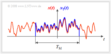
For the ACF and PDS calculation of a random signal

- The power density spectrum ${\it Φ}_x(f)$ can be given – as well as the auto-correlation function $φ_x(τ)$ – for each individual pattern function of the stationary and ergodic random process $\{x(t)\}$, even if the specific course of $x(t)$ is explicitly unknown.
- The amplitude spectrum $X(f)$, on the other hand, is undefined because if the spectral function $X(f)$ is known, the entire time function $x(t)$ from $–∞$ to $+∞$ would also have to be known via the Fourier inverse transform, which clearly cannot be the case for a stochastic signal.
- If a time section of the finite time duration $T_{\rm M}$ is known according to the sketch on the left, the Fourier transform can of course be applied to it again.
$\text{Theorem:}$ The following relationship exists between the power density spectrum ${\it Φ}_x(f)$ of the infinite time random signal $x(t)$ and the amplitude spectrum $X_{\rm T}(f)$ of the finite time section $x_{\rm T}(t)$:
- $${ {\it \Phi}_x(f)} = \lim_{T_{\rm M}\to\infty}\hspace{0.2cm}
\frac{1}{ T_{\rm M} }\cdot \vert X_{\rm T}(f)\vert ^2.$$
$\text{Proof:}$ Previously, the auto-correlation function of an ergodic process with the sample function $x(t)$ was given as follows:
- $${ {\it \varphi}_x(\tau)} = \lim_{T_{\rm M}\to\infty}\hspace{0.2cm}
\frac{1}{ T_{\rm M} }\cdot\int^{+T_{\rm M}/2}_{-T_{\rm M}/2}x(t)\cdot x(t + \tau)\hspace{0.1cm} \rm d \it t.$$
- It is permissible to replace the function $x(t)$, which is unbounded in time, by the function $x_{\rm T}(t)$, which is bounded on the time range $-T_{\rm M}/2$ to $+T_{\rm M}/2$. $x_{\rm T}(t)$ corresponds to the spectrum $X_{\rm T}(f)$, and by applying the first Fourier integral and the shifting theorem:
- $${ {\it \varphi}_x(\tau)} = \lim_{T_{\rm M}\to\infty}\hspace{0.2cm}
\frac{1}{ T_{\rm M} }\cdot \int^{+T_{\rm M}/2}_{-T_{\rm M}/2}x_{\rm T}(t)\cdot \int^{+\infty}_{-\infty}X_{\rm T}(f)\cdot {\rm e}^{ {\rm j}2 \pi f ( t + \tau) } \hspace{0.1cm} \rm d \it f \hspace{0.1cm} \rm d \it t.$$
- After splitting the exponent and swapping the time and frequency integrals, we get:
- $${ {\it \varphi}_x(\tau)} = \lim_{T_{\rm M}\to\infty}\hspace{0.2cm}
\frac{1}{ T_{\rm M} }\cdot \int^{+\infty}_{-\infty}X_{\rm T}(f)\cdot \left[ \int^{+T_{\rm M}/2}_{-T_{\rm M}/2}x_{\rm T}(t)\cdot {\rm e}^{ {\rm j}2 \pi f t } \hspace{0.1cm} \rm d \it t \right] \cdot {\rm e}^{ {\rm j}2 \pi f \tau} \hspace{0.1cm} \rm d \it f.$$
- The inner integral describes the conjugate-complex spectrum $X_{\rm T}^{\star}(f)$. It further follows that:
- $${ {\it \varphi}_x(\tau)} = \lim_{T_{\rm M}\to\infty}\hspace{0.2cm}
\frac{1}{ T_{\rm M} }\cdot \int^{+\infty}_{-\infty}\vert X_{\rm T}(f)\vert^2 \cdot {\rm e}^{ {\rm j}2 \pi f \tau} \hspace{0.1cm} \rm d \it f.$$
- A comparison with Wiener and Chintchin's theorem which is always valid in ergodicity,
- $${ {\it \varphi}_x(\tau)} = \int^{+\infty}_{-\infty}{\it \Phi}_x(f)
\cdot {\rm e}^{ {\rm j}2 \pi f \tau} \hspace{0.1cm} \rm d \it f ,$$
- shows the validity of the above relation:
- $${ {\it \Phi}_x(f)} = \lim_{T_{\rm M}\to\infty}\hspace{0.2cm}
\frac{1}{ T_{\rm M} }\cdot \vert X_{\rm T}(f)\vert^2.$$
Power density spectrum of the filter output signal
Combining the statements made in the last two sections, we arrive at the following important result:
$\text{Theorem:}$ The power density spectrum (PDS) at the output of a linear time-invariant system with frequency response $H(f)$ is obtained as the product of the input PDS ${\it Φ}_x(f)$ and the "power transfer function" $\vert H(f)\vert ^2$.
- $${ {\it \Phi}_y(f)} = { {\it \Phi}_x(f)} \cdot \vert H(f)\vert ^2.$$
$\text{Proof:}$ Starting from the three relations already derived before:
- $${ {\it \Phi}_x(f)} =\hspace{-0.1cm} \lim_{T_{\rm M}\to\infty}\hspace{0.01cm}
\frac{1}{ T_{\rm M} }\hspace{-0.05cm}\cdot\hspace{-0.05cm} \vert X_{\rm T}(f)\vert^2, \hspace{0.5cm} { {\it \Phi}_y(f)} =\hspace{-0.1cm} \lim_{T_{\rm M}\to\infty}\hspace{0.01cm} \frac{1}{ T_{\rm M} }\hspace{-0.05cm}\cdot\hspace{-0.05cm}\vert Y_{\rm T}(f)\vert^2, \hspace{0.5cm} Y_{\rm T}(f) = X_{\rm T}(f) \hspace{-0.05cm}\cdot\hspace{-0.05cm} H(f).$$ Substituting these equations into each other, we get the above result.
The following example illustrates the relationship with white noise.

$\text{Example 1:}$ At the input of a Gaussian low-pass filter with the frequency response
- $$H(f) = {\rm e}^{- \pi \hspace{0.03cm}\cdot \hspace{0.03cm}(f/\Delta f)^2}$$
white noise $x(t)$ with noise power density ${ {\it \Phi}_x(f)} =N_0/2$ is present ⇒ two-sided representation. Then, the following holds for the power density spectrum of the output signal:
- $${ {\it \Phi}_y(f)} = \frac {N_0}{2} \cdot {\rm e}^{- 2 \pi \hspace{0.03cm}\cdot \hspace{0.03cm}(f/\Delta
f)^2}.$$ The diagram shows the signals and power density spectra at the filter input and output.
Notes:
- The signal $x(t)$ – strictly speaking – cannot be plotted at all, since it has an infinite power ⇒ integral over ${\it Φ}_x(f)$ from $-\infty$ to $+\infty$.
- The output signal $y(t)$ has a lower frequency than $x(t)$ and a finite power corresponding to the integral over ${\it Φ}_y(f)$.
- In one-sided representation, (only) for $f>0$ would hold: ${ {\it \Phi}_x(f)} =N_0$. he statements (1) and (2) would also apply here in the same way.
The auto-correlation function of the filter output signal
The calculated power density spectrum (PDS) can also be written as follows:
- $${{\it \Phi}_y(f)} = {{\it \Phi}_x(f)} \cdot H(f) \cdot H^{\star}(f)$$
$\text{Theorem:}$ The corresponding auto-correlation function (ACF) is then obtained according to the regularities of the Fourier transform and by applying the convolution theorem:
- $${ {\it \varphi}_y(\tau)} = { {\it \varphi}_x(\tau)} \ast h(\tau)\ast h(-
\tau).$$
In the transition from the spectral to the time domain, note:
- The Fourier retransforms are to be inserted in each case, namely
- $${{\it \varphi}_y(\tau)} \circ\hspace{0.05cm}\!\!\!-\!\!\!-\!\!\!-\!\!\bullet\,{{\it \Phi}_y(f)}, \hspace{0.5cm}{{\it \varphi}_x(\tau)} \circ\hspace{0.05cm}\!\!\!-\!\!\!-\!\!\!-\!\!\!\bullet\,{{\it \Phi}_x(f)}, \hspace{0.5cm}{h(\tau)} \circ\hspace{0.05cm}\!\!\!-\!\!\!-\!\!\!-\!\!\bullet\,{H(f)}, \hspace{0.5cm}{h(-\tau)} \circ\hspace{0.05cm}\!\!\!-\!\!\!-\!\!\!-\!\!\!\bullet\,{H^{\star}(f)}$$
- Moreover, each multiplication becomes a convolution operation.

$\text{Example 2:}$ We consider again the same scenario as in $\text{Example 1}$, but this time in the time domain:
- white noise ${ {\it \Phi}_x(f)} =N_0/2$,
- Gaussian filter: $H(f) = {\rm e}^{- \pi \hspace{0.03cm}\cdot \hspace{0.03cm}(f/\Delta f)^2}\hspace{0.3cm}\Rightarrow \hspace{0.3cm}
h(t) = \Delta f \cdot {\rm e}^{- \pi \hspace{0.03cm}\cdot \hspace{0.03cm}(\Delta f \hspace{0.03cm}\cdot \hspace{0.03cm}t)^2}.$
One can see from this diagram:
- The ACF of the input signal is now a Dirac function with weight $N_0/2$.
- By convolution twice with the (here also Gaussian) impulse response $h(t)$ or $h(–t)$ one obtains the ACF $φ_y(τ)$ of the output signal.
- Thus, the ACF $φ_y(τ)$ of the output signal is also Gaussian.
- The ACF value at $τ = 0$ is identical to the area of the power density spectrum ${\it Φ}_y(f)$ and characterizes the signal power (variance) $σ_y^2$.
- In contrast, the area at $φ_y(τ)$ gives the PDS value ${\it Φ}_y(f = \rm 0)$, i.e., $N_0/2$.
Cross correlation function between input and output signal

We again consider a filter with the frequency response $H(f)$ and the impulse response $h(t)$. Further applies:
- The stochastic input signal $x(t)$ is a sample function of the ergodic random process $\{x(t)\}$.
- The corresponding auto-correlation function (ACF) at the filter input is thus $φ_x(τ)$, while the power density spectrum (PDS) is denoted by ${\it Φ}_x(f)$.
- The corresponding descriptors of the ergodic random process $\{y(t)\}$ at the filter output are the sample function $y(t)$, the auto-correlation function $φ_y(τ)$ and the conductance density spectrum ${\it Φ}_y(f)$.
$\text{Theorem:}$ For the cross correlation function (CCF) between the input and the output signal holds:
- $${ {\it \varphi}_{xy}(\tau)} = h(\tau)\ast { {\it \varphi}_x(\tau)} .$$
Here, $h(τ)$ denotes the impulse response of the filter $($with the time variable $τ$ instead of $t)$ and ${ {\it \varphi}_{x}(\tau)}$ denotes the ACF of the input signal.
$\text{Proof:}$ In general, for the cross-correlation function between two signals $x(t)$ and $y(t)$:
- $${ {\it \varphi}_{xy}(\tau)} = \lim_{T_{\rm M}\to\infty}\hspace{0.2cm}\frac{1}{ T_{\rm M} }\cdot\int^{+T_{\rm M}/2}_{-T_{\rm M}/2}x(t)\cdot y(t + \tau)\hspace{0.1cm} \rm d \it t.$$
- With the generally valid relation $y(t) = h(t) \ast x(t)$ and the formal integration variable $θ$, we can also write for this:
- $${ {\it \varphi}_{xy}(\tau)} = \lim_{T_{\rm M}\to\infty}\hspace{0.2cm}\frac{1}{ T_{\rm M} }\cdot\int^{+T_{\rm M}/2}_{-T_{\rm M}/2}x(t)\cdot \int^{+\infty}_{-\infty} h(\theta) \cdot x(t + \tau - \theta)\hspace{0.1cm}{\rm d}\theta\hspace{0.1cm}{\rm d} \it t.$$
- By interchanging the two integrals and subtracting the limit into the integral, we obtain:
- $${ {\it \varphi}_{xy}(\tau)} = \int^{+\infty}_{-\infty}
h(\theta) \cdot \left[ \lim_{T_{\rm M}\to\infty}\hspace{0.2cm} \frac{1}{ T_{\rm M} } \cdot\int^{+T_{\rm M}/2}_{-T_{\rm M}/2}x(t)\cdot x(t + \tau - \theta)\hspace{0.1cm} \hspace{0.1cm} {\rm d} t \right]{\rm d}\theta.$$
- The expression in the square brackets gives the ACF value at the input at time $τ - θ$:
- $${ {\it \varphi}_{xy}(\tau)} = \int^{+\infty}_{-\infty}h(\theta) \cdot \varphi_x(\tau - \theta)\hspace{0.1cm}\hspace{0.1cm} {\rm d}\theta = h(\tau)\ast { {\it \varphi}_x(\tau)} .$$
- However, the remaining integral describes the convolution operation in detailed notation.
$\text{Conclusion:}$ In the frequency domain, the corresponding equation is:
- $${ {\it \Phi}_{xy}(f)} = H(f)\cdot{ {\it \Phi}_x(f)} \hspace{0.3cm} \Rightarrow \hspace{0.3cm} H(f) = \frac{ {\it \Phi}_{xy}(f)}{ {\it \Phi}_{x}(f)}.$$
This equation shows that the filter frequency response $H(f)$ from a measurement with stochastic excitation can be calculated completely – i.e., both magnitude and phase – if the following descriptive quantities are determined:
- the statistical characteristics at the input, either the ACF $φ_x(τ)$ or the PDS ${\it Φ}_x(f)$,
- as well as the cross correlation function $φ_{xy}(τ)$ or its Fourier transform ${\it Φ}_{xy}(f)$.
Exercises for the chapter
Exercise 5.1: Gaussian ACF and Gaussian Low-Pass
Exercise 5.1Z: $\cos^2$ Noise Limitation
Exercise 5.2: Determination of the Frequency Response
Exercise 5.2Z: Two-Way Channel
