Aufgaben:Exercise 5.1Z: Cosine Square Noise Limitation

• Return to book

Top:  Input PDS  ${\it Φ}_x(f)$,
Bottom:  Filter frequency response $H(f)$

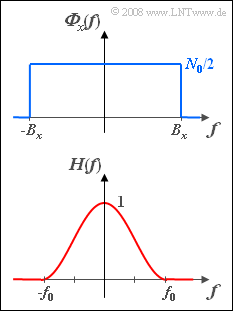
We consider bandlimited white noise  $x(t)$  with the power density spectrum  ${\it Φ}_x(f)$  sketched above. This is constant equal to  $N_0/2$  in the range  $|f| \le B_x$  and zero outside.

Assume the following numerical values:

• Noise power density  $N_0 = 10^{-16} \ \rm V^2/Hz$,
• (one-sided) noise bandwidth  $B_x = 10 \ \rm kHz$.

This signal is applied to the input of a low-pass filter with frequency response $$H(f) = \left\{ {\begin{array}{*{20}c} {\cos ^2 \left( {\frac{{{\rm{\pi }}f}}{2f_0 }} \right)} & {\rm{f\ddot{u}r}\quad \left| \it f \right| \le \it f_{\rm 0} ,} \\ 0 & {{\rm{else}}} \\\end{array}} \right.$$

  Here  $f_0$  denotes the absolute filter bandwidth, which can vary between  $B_x/2$  and  $2B_x$. 

The filter output signal is denoted by  $y(t)$. 

Notes:

• The exercise belongs to the chapter  Stochastic System Theory.
• Reference is also made to the chapters  Gaussian Distributed Random Variables  and  Power Density Spectrum.

• Use the following equations if necessary:

$${\rm Q}(x) \approx \frac{1}{{\sqrt {2{\rm{\pi }}} \cdot x}} \cdot {\rm{e}}^{ - x^2 /2} \hspace{0.15cm}( \text{für große }x),$$

$$\int {\rm{cos}}^{\rm{2}}( {ax} )\hspace{0.1cm}{\rm{d}}x = \frac{1}{2} \cdot x + \frac{1}{4a} \cdot \sin ( {2ax} ),$$

$$\int {\cos ^4 } ( {ax} )\hspace{0.1cm}{\rm{d}}x = \frac{3}{8} \cdot x + \frac{1}{4a} \cdot \sin ( {2ax} ) + \frac{1}{32a} \cdot \sin ( {4ax} ).$$

Questions

1

What is the rms value of the input signal  $x(t)$?

$\sigma_x \ = \ $ $\ \rm µ V$

2

What is the probability that an instantaneous voltage value of the input signal is greater than  $5 \hspace{0.05cm} \rm µ V$  in magnitude?

${\rm Pr}(|x(t)| > 5 \hspace{0.05cm} \rm µ V) \ = \ $ $\ \cdot 10^{-6}$

3

What is the mean value (DC component) of the output signal  $y(t)$?

$m_y\ \ = \ $ $\ \rm µ V$

4

Calculate the rms value of the output signal  $y(t)$  for  $f_0 = B_x/2$.

$\sigma_y \ = \ $ $\ \rm µ V$

5

Calculate the rms value of  $y(t)$  under the condition  $f_0 = 2 \cdot B_x$.

$\sigma_y \ = \ $ $\ \rm µ V$

6

Let  $f_0 = 2 \cdot B_x$  be further valid. What is the probability that the output signal  $y(t)$  is greater than  $5 \hspace{0.05cm} \rm µ V$  in magnitude?

${\rm Pr}(|y(t)| > 5 \hspace{0.05cm} \rm µ V) \ = \ $ $\ \cdot 10^{-12}$

Solution

Solution

(1)  The variance (power)   ⇒   rms squared of the signal  $x(t)$  is

$$\sigma _x ^2 = \frac{N_0 }{2} \cdot 2B_x = N_0 \cdot B_x = 10^{ - 12} \;{\rm{V}}^2 \hspace{0.3cm}\Rightarrow\hspace{0.3cm} \sigma _x \hspace{0.15cm}\underline{ = 1\,\,{\rm µ}{\rm V}}.$$

(2)  According to the chapter "Gaussian Distributed Random Variables" and the approximation given here  $($for large  $x)$,  we obtain:

$$\Pr \left( {\left| {x(t)} \right| > 5\;{\rm{µ V}}} \right) = 2 \cdot {\rm Q}(5) = \frac{2}{{\sqrt {2{\rm{\pi }}} \cdot 5}} \cdot {\rm{e}}^{ - 12.5}\hspace{0.15cm} \underline{ \approx 0.6 \cdot 10^{ - 6}} .$$

(3)  The input signal  $x(t)$  is mean-free  $(m_x = 0)$.

• Otherwise  ${\it Φ}_x(f)$  would still have to contain a Dirac function at  $f= 0$. 
• The mean is not changed by the linear filter   ⇒   $m_y\hspace{0.05cm}\underline{ = 0}$.

(4)  For the power density spectrum of the output signal generally applies:

$${\it \Phi}_y (f) = {N_0 }/{2} \cdot \left| {H( f )} \right|^2 .$$

• Thus, the variance  $\sigma _y^2$  can be calculated.  Taking advantage of the symmetry, we obtain:

$$\sigma _y ^2 = {N_0 }/{2} \cdot \int_{ - \infty }^{ + \infty } {\left| {H( f )} \right|^2 \hspace{0.1cm}{\rm{d}}f} = N_0 \cdot \int_0^{f_0 } {\cos ^4 } \left( {\frac{{{\rm{\pi }}f}}{2f_0 }} \right)\hspace{0.1cm}{\rm{d}}f .$$

• The definite integral is given.  For each of the three solution terms, the value of the lower bound is zero.  It follows that:

$$\sigma _y ^2 = {N_0}/{2} \cdot \left( {\frac{3}{8} \cdot f_0 + \frac{f_0 }{{2{\rm{\pi }}}} \cdot \sin ( {\rm{\pi }} ) + \frac{f_0 }{{16{\rm{\pi }}}} \cdot \sin ( {{\rm{2\pi }}} )} \right) = \frac{3}{8} \cdot N_0 \cdot f_0 $$

$$\Rightarrow \hspace{0.3cm} f_0 = B_x/2\text{:}\hspace{0.2cm}\sigma _y ^2 = \frac{3}{16} \cdot N_0 \cdot B_x = \frac{3}{16} \cdot \sigma _x ^2 = 0.1875 \cdot 10^{ - 12} \;{\rm{V}}^2 \hspace{0.2cm}\Rightarrow \hspace{0.2cm}\sigma _y \hspace{0.15cm}\underline{ = 0.433\;{\rm{µ V}}}{\rm{.}}$$

(5)  Now the input PDS for  $|f| > B_x$  has no components.

• Therefore holds:

$$\sigma _y ^2 = N_0\cdot \int_0^{B_x } {\cos ^4 \left( {\frac{{{\rm{\pi }}f}}{2f_0 }} \right)\hspace{0.1cm}{\rm{d}}f = N_0 \cdot \int_0^{f_0 /2} {\cos ^4 } \left( {\frac{{{\rm{\pi }}f}}{2f_0 }} \right)\hspace{0.1cm}{\rm{d}}f.}$$

• The numerical evaluation yields for this:

$$\sigma _y ^2 = N_0 \left( {\frac{3}{8} \cdot B_x + \frac{B_x }{{2{\rm{\pi }}}} \cdot \sin ( {\frac{{\rm{\pi }}}{2}} ) + \frac{B_x }{{{\rm{16\pi }}}} \cdot \sin ( {\rm{\pi }} )} \right) = N_0 \cdot B_x \left( {\frac{3}{8} + \frac{1}{{2{\rm{\pi }}}}} \right) = 0.534\cdot \sigma _x ^2 \hspace{0.3cm}\Rightarrow \hspace{0.3cm}\sigma _y \hspace{0.15cm}\underline{ = 0.731\;{\rm{µ V}}}{\rm{.}}$$

(6)  Analogous to the sample solution of subtask  (2)  holds:

$$\Pr \left( {\left| {y\left( t \right)} \right| > 5\;{\rm{µ V}}} \right) = 2 \cdot {\rm Q}\left( {\frac{{5\;{\rm{µ V}}}}{{0.731\;{\rm{µ V}}}}} \right) = 2 \cdot {\rm Q}( {6.84} ).$$

• With the given approximation, this probability has the following value:

$$\Pr \left( {\left| {y\left( t \right)} \right| > 5\;{\rm{µ V}}} \right) \hspace{0.15cm} \underline{ \approx 8 \cdot 10^{ - 12}}.$$