Aufgaben:Exercise 2.5: Ternary Signal Transmission

• Return to book

Probability density function of a noisy ternary signal

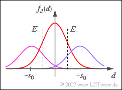
A ternary transmission system  $(M = 3)$  with the possible amplitude values  $-s_0$,  $0$  and  $+s_0$ is considered.

• During transmission, additive Gaussian noise with rms value  $\sigma_d$ is added to the signal.
• The recovery of the three-level digital signal at the receiver is done with the help of two decision thresholds at  $E_{–}$  and  $E_{+}$.

• First, the occurrence probabilities of the three input symbols are assumed to be equally probable:

$$p_{\rm -} = {\rm Pr}(-s_0) = {1}/{ 3}, \hspace{0.15cm} p_{\rm 0} = {\rm Pr}(0) = {1}/{ 3}, \hspace{0.15cm} p_{\rm +} = {\rm Pr}(+s_0) ={1}/{ 3}\hspace{0.05cm}.$$

• For the time being, the decision thresholds are centered at  $E_{–} = \, –s_0/2$ and $E_{+} = +s_0/2$.

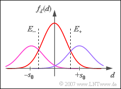
From subtask (3) on, the symbol probabilities are  $p_{–} = p_+ = 1/4$  and  $p_0 = 1/2$, as shown in the diagram. For this constellation, the symbol error probability  $p_{\rm S}$  is to be minimized by varying the decision thresholds  $E_{–}$  and  $E_+$. 

Notes:

• The exercise refers to the chapter  "Redundancy-Free Coding".
• For the symbol error probability  $p_{\rm S}$  of a  $M$–level message transmission system with equally probable input symbols and threshold values exactly in the middle between two adjacent amplitude levels holds:

$$p_{\rm S} = \frac{ 2 \cdot (M-1)}{M} \cdot {\rm Q} \left( {\frac{s_0}{(M-1) \cdot \sigma_d}}\right) \hspace{0.05cm}.$$

• You can numerically determine the error probability values according to the  ${\rm Q}$ or  ${\rm erfc}$ function using the  "Complementary Gaussian Error Functions"  interaction module.
• To check the results, use the calculation module  "Symbol error probability of digital communications systems".

Questions

1

What symbol error probability results with the (normalized) noise rms value  $\sigma_d/s_0 = 0.25$  for equally probable symbols?

$p_0 = 1/3, \ \sigma_d = 0.25 \text{:} \hspace{0.4cm} p_{\rm S} \ = \ $ $\ \%$

2

How does the symbol error probability change with  $\sigma_d/s_0 = 0.5$?

$p_0 = 1/3, \ \sigma_d = 0.5 \text{:} \hspace{0.4cm} p_{\rm S} \ = \ $ $\ \%$

3

What value results with  $p_{–} = p_+ = 0.25$  and  $p_0 = 0.5$?

$p_0 = 1/2, \ \sigma_d = 0.5 \text{:} \hspace{0.4cm} p_{\rm S} \ = \ $ $\ \%$

4

Determine the optimal thresholds  $E_+$  and  $E_{–} = \, –E_+$  for  $p_0 = 1/2$.

$p_0 = 1/2, \ \sigma_d = 0.5 \text{:} \hspace{0.4cm} E_{\rm +, \ opt} \ = \ $

5

What is the probability of error for optimal thresholds?

${\rm optimal \ thresholds} \text{:} \hspace{0.4cm} p_{\rm S} \ = \ $ $\ \%$

6

What are the optimal thresholds for  $p_0 = 0.2$  and $ p_{–} = p_+ = 0.4$?

$p_0 = 0.2, \ \sigma_d = 0.5 \text{:} \hspace{0.4cm} E_{\rm +, \ opt} \ = \ $

7

What is the symbol error probability now? Interpretation.

${\rm optimal \ thresholds} \text{:} \hspace{0.4cm} p_{\rm S} \ = \ $ $\ \%$

Solution

Solution

(1)  According to the given equation, with $M = 3$ and $\sigma_d/s_0 = 0.25$:

$$p_{\rm S} = \frac{ 2 \cdot (M-1)}{M} \cdot {\rm Q} \left( {\frac{s_0}{(M-1) \cdot \sigma_d}}\right)= {4}/{ 3}\cdot {\rm Q}(2) ={4}/{ 3}\cdot 0.0228\hspace{0.15cm}\underline {\approx 3 \,\%} \hspace{0.05cm}.$$

(2)  When the noise rms value is doubled, the error probability also increases significantly:

$$p_{\rm S} = {4}/{ 3}\cdot {\rm Q}(1)= {4}/{ 3}\cdot 0.1587 \hspace{0.15cm}\underline {\approx 21.2 \,\%} \hspace{0.05cm}.$$

(3)  The two outer symbols are each distorted with probability $p = {\rm Q}(s_0/(2 \cdot \sigma_d)) = 0.1587$.

• The distortion probability of the symbol  $0$  is twice as large (it is limited by two thresholds).
• Considering the individual symbol probabilities, we obtain:

$$p_{\rm S} = {1}/{ 4}\cdot p + {1}/{ 2}\cdot 2p +{1}/{ 4}\cdot p = 1.5 \cdot p = 1.5 \cdot 0.1587 \hspace{0.15cm}\underline {\approx 23.8 \,\%} \hspace{0.05cm}.$$

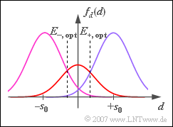
(4)  Since the symbol  $0$  occurs more frequently and can also be biased in both directions, the thresholds should be shifted outward.

• The optimal decision threshold $E_{\rm +, \ opt}$ is obtained from the intersection of the two Gaussian functions shown in the graph. It must hold:

Optimal thresholds for (4)

$$\frac{ 1/2}{ \sqrt{2\pi} \cdot \sigma_d} \cdot {\rm exp} \left[ - \frac{ E_{\rm +}^2}{2 \cdot \sigma_d^2}\right] = \frac{ 1/4}{ \sqrt{2\pi} \cdot \sigma_d} \cdot {\rm exp} \left[ - \frac{ (s_0 -E_{\rm +})^2}{2 \cdot \sigma_d^2}\right]$$

$$\Rightarrow \hspace{0.3cm} {\rm exp} \left[ \frac{ (s_0 -E_{\rm +})^2 - E_{\rm +}^2}{2 \cdot \sigma_d^2}\right]= {1}/{ 2} \Rightarrow \hspace{0.3cm} {\rm exp} \left[ \frac{ 1 -2 \cdot E_{\rm +}/s_0}{2 \cdot \sigma_d^2/s_0^2}\right]= {1}/{ 2}$$

$$\Rightarrow \hspace{0.3cm}\frac{ E_{\rm +}}{s_0}= \frac{1} { 2}+ \frac{\sigma_d^2} {s_0^2} \cdot {\rm ln}(2)\hspace{0.15cm}\underline {=0.673}\hspace{0.15cm}\approx {2}/ {3} \hspace{0.05cm}.$$

(5)  Using the approximate result from (4), we obtain:

$$p_{\rm S} \ = \ { 1}/{4} \cdot {\rm Q} \left( {\frac{s_0/3}{ \sigma_d}}\right)+ 2 \cdot { 1}/{2} \cdot {\rm Q} \left( {\frac{2s_0/3}{ \sigma_d}}\right) +{ 1}/{4} \cdot {\rm Q} \left( {\frac{s_0/3}{ \sigma_d}}\right)$$

$$\Rightarrow \hspace{0.3cm}p_{\rm S} \ = \ = { 1}/{2} \cdot {\rm Q} \left( 2/3 \right)+ {\rm Q} \left( 4/3 \right)= { 1}/{2} \cdot 0.251 + 0.092 \hspace{0.15cm}\underline {\approx 21.7 \,\%} \hspace{0.05cm}.$$

Optimal thresholds for (6)

(6)  After a similar calculation as in point (4) we get

• $E_+ = 1 \, –0.0673 \ \underline{= 0.327} \approx 1/3$.
• $E_{–} = \, –E_+$ is still valid.

(7)  Similar to the sample solution for subtask (5), one now obtains:

$$p_{\rm S} \ = \ 0.4 \cdot {\rm Q} \left( 4/3 \right)+ 2 \cdot 0.2 \cdot{\rm Q} \left( 2/3 \right)+0.4 \cdot {\rm Q} \left( 4/3 \right)$$

$$\Rightarrow \hspace{0.3cm}p_{\rm S} \ = \ 0.4 \cdot (0.092 + 0.251 + 0.092) \hspace{0.15cm}\underline {\approx 17.4 \,\%} \hspace{0.05cm}.$$

Discussion of the result:

• Accordingly, there is a smaller symbol error probability ($17.4 \ \%$ versus $21.2 \ \%$) than with equal probability amplitude coefficients.
• However, redundancy-free coding is no longer present, even if the amplitude coefficients are statistically independent of each other.
• While for equally probable ternary symbols the entropy is $H = {\rm log}_2(3) = 1.585 \ {\rm bit/ternary \ symbol}$ beträgt   ⇒   equivalent bit rate (the information flow) $R_{\rm B} = H/T$, with probabilities $p_0 = 0.2$ and $p_{–} = p_+ = 0.4$:

$$H \ = \ 0.2 \cdot {\rm log_2} (5) + 2 \cdot 0.4 \cdot {\rm log_2} (2.5)= 0.2 \cdot 2.322 + 0.8 \cdot 1.322 \hspace{0.15cm}\underline {\approx 1.522\,\, {\rm bit/ternary \ symbol}} \hspace{0.05cm}.$$

• Thus, the equivalent bit rate is $4 \ \%$ smaller than the maximum possible for $M = 3$.