Difference between revisions of "Aufgaben:Exercise 4.07: Decision Boundaries once again"
| Line 1: | Line 1: | ||
| − | {{quiz-Header|Buchseite= | + | {{quiz-Header|Buchseite=Digital_Signal_Transmission/Approximation_of_the_Error_Probability}} |
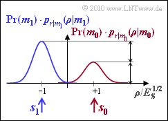
| − | [[File:P_ID2017__Dig_A_4_7.png|right|frame| | + | [[File:P_ID2017__Dig_A_4_7.png|right|frame|PDF with unequal symbol probabilities]] |
| − | + | We consider a transmission system with | |
| − | * | + | * only one basis function $(N = 1)$, |
| − | * | + | * two signals $(M = 2)$ with $s_0 = \sqrt{E_s}$ and $s_1 = -\sqrt{E_s}$ , |
| − | * | + | * an AWGN channel with variance $\sigma_n^2 = N_0/2$. |
| − | + | Since this exercise deals with the general case ${\rm Pr}(m_0) ≠ {\rm Pr}(m_1)$, it is not sufficient to consider the conditional density functions $p_{\it r\hspace{0.05cm}|\hspace{0.05cm}m_i}(\rho\hspace{0.05cm} |\hspace{0.05cm}m_i)$. Rather, these must still be multiplied by the symbol probabilities ${\rm Pr}(m_i)$. For $i$, the values $0$ and $1$ have to be used here. | |
| − | + | If the decision boundary between the two regions $I_0$ and $I_1$ is at $G = 0$, i.e., in the middle between $\boldsymbol{s}_0$ and $\boldsymbol{s}_1$, the error probability is independent of the occurrence probabilities ${\rm Pr}(m_0)$ and ${\rm Pr}(m_1)$: | |
:$$p_{\rm S} = {\rm Pr}({ \cal E} ) = {\rm Q} \left ( \frac{d/2}{\sigma_n} \right ) \hspace{0.05cm}.$$ | :$$p_{\rm S} = {\rm Pr}({ \cal E} ) = {\rm Q} \left ( \frac{d/2}{\sigma_n} \right ) \hspace{0.05cm}.$$ | ||
| − | + | Here $d$ indicates the distance between the signal points $s_0$ and $s_1$ and $d/2$ accordingly the respective distance of $s_0$ and $s_1$ from the decision boundary $G = 0$. The rms value (root of the variance) of the AWGN noise is $\sigma_n$. | |
| − | + | If, on the other hand, the occurrence probabilities are different ⇒ ${\rm Pr}(m_0) ≠ {\rm Pr}(m_1)$, a smaller error probability can be obtained by shifting the decision boundary $G$: | |
:$$p_{\rm S} = {\rm Pr}(m_1) \cdot {\rm Q} \left ( \frac{d/2}{\sigma_n} \cdot (1 + \gamma) \right ) | :$$p_{\rm S} = {\rm Pr}(m_1) \cdot {\rm Q} \left ( \frac{d/2}{\sigma_n} \cdot (1 + \gamma) \right ) | ||
+ {\rm Pr}(m_0) \cdot {\rm Q} \left ( \frac{d/2}{\sigma_n} \cdot (1 - \gamma) \right )\hspace{0.05cm},$$ | + {\rm Pr}(m_0) \cdot {\rm Q} \left ( \frac{d/2}{\sigma_n} \cdot (1 - \gamma) \right )\hspace{0.05cm},$$ | ||
| − | + | where the auxiliary quantity $\gamma$ is defined as follows: | |
:$$\gamma = 2 \cdot \frac{ \sigma_n^2}{d^2} \cdot {\rm ln} \hspace{0.15cm} \frac{{\rm Pr}( m_1)}{{\rm Pr}( m_0)} | :$$\gamma = 2 \cdot \frac{ \sigma_n^2}{d^2} \cdot {\rm ln} \hspace{0.15cm} \frac{{\rm Pr}( m_1)}{{\rm Pr}( m_0)} | ||
\hspace{0.05cm},\hspace{0.2cm} G_{\rm opt} = \gamma \cdot \sqrt {E_{\rm S}}\hspace{0.05cm}.$$ | \hspace{0.05cm},\hspace{0.2cm} G_{\rm opt} = \gamma \cdot \sqrt {E_{\rm S}}\hspace{0.05cm}.$$ | ||
| Line 26: | Line 26: | ||
| − | '' | + | ''Notes:'' |
| − | * | + | * The exercise belongs to the chapter [[Digital_Signal_Transmission/Approximation_of_the_Error_Probability|"Approximation of the Error Probability"]]. |
| − | * | + | * You can find the values of the Q–function with interactive applet [[Applets:Komplementäre_Gaußsche_Fehlerfunktionen|"Complementary Gaussian Error Functions"]]. |
| − | === | + | ===Questions=== |
<quiz display=simple> | <quiz display=simple> | ||
| − | { | + | {What are the underlying symbol probabilities of the graph, if the blue Gaussian curve is exactly twice as high as the red one? |
|type="{}"} | |type="{}"} | ||
${\rm Pr}(m_0)\ = \ $ { 0.333 3% } | ${\rm Pr}(m_0)\ = \ $ { 0.333 3% } | ||
${\rm Pr}(m_1)\ = \ $ { 0.667 3% } | ${\rm Pr}(m_1)\ = \ $ { 0.667 3% } | ||
| − | { | + | {What is the error probability with noise variance $\sigma_n^2 = E_{\rm S}/9$ and the '''given threshold''' $G = 0$? |
|type="{}"} | |type="{}"} | ||
$G = 0 \text{:} \hspace{0.85cm} p_{\rm S} \ = \ $ { 0.135 3% } $\ \%$ | $G = 0 \text{:} \hspace{0.85cm} p_{\rm S} \ = \ $ { 0.135 3% } $\ \%$ | ||
| − | { | + | {What is the optimal threshold for the given probabilities? |
|type="{}"} | |type="{}"} | ||
$G_{\rm opt}\ = \ $ { 0.04 3% } $\ \cdot \sqrt{E_s}$ | $G_{\rm opt}\ = \ $ { 0.04 3% } $\ \cdot \sqrt{E_s}$ | ||
| − | { | + | {What is the probability of error for '''optimal threshold''' $G = G_{\rm opt}$? |
|type="{}"} | |type="{}"} | ||
$G = G_{\rm opt} \text{:} \hspace{0.2cm} p_{\rm S}\ = \ $ { 0.126 3% } $\ \%$ | $G = G_{\rm opt} \text{:} \hspace{0.2cm} p_{\rm S}\ = \ $ { 0.126 3% } $\ \%$ | ||
| − | { | + | {What error probabilities are obtained with the noise variance $\sigma_n^2 = E_{\rm S}$? |
|type="{}"} | |type="{}"} | ||
$G = 0 \text{:} \hspace{0.85cm} p_{\rm S}\ = \ $ { 15.9 3% } $\ \%$ | $G = 0 \text{:} \hspace{0.85cm} p_{\rm S}\ = \ $ { 15.9 3% } $\ \%$ | ||
$G = G_{\rm opt} \text{:} \hspace{0.2cm} p_{\rm S}\ = \ $ { 14.5 3% } $\ \%$ | $G = G_{\rm opt} \text{:} \hspace{0.2cm} p_{\rm S}\ = \ $ { 14.5 3% } $\ \%$ | ||
| − | { | + | {Which statements are true for the noise variance $\sigma_n^2 = 4 \cdot E_{\rm S}$? |
|type="[]"} | |type="[]"} | ||
| − | + | + | + With $G = 0$, the probability of error is greater than $30\%$. |
| − | + | + | + The optimal decision threshold is to the right of $s_0$. |
| − | + | + | + With optimal threshold, the error probability is about $27\%$. |
| − | + | + | + The estimated value $m_0$ is possible only with sufficiently large noise. |
</quiz> | </quiz> | ||
| − | === | + | ===Solution=== |
{{ML-Kopf}} | {{ML-Kopf}} | ||
| − | '''(1)''' | + | '''(1)''' The heights of the two drawn density functions are proportional to the occurrence probabilities ${\rm Pr}(m_0)$ and ${\rm Pr}(m_1)$. From |
:$${\rm Pr}(m_1) = 2 \cdot {\rm Pr}(m_0) \hspace{0.05cm},\hspace{0.2cm} {\rm Pr}(m_0) + {\rm Pr}(m_1) = 1$$ | :$${\rm Pr}(m_1) = 2 \cdot {\rm Pr}(m_0) \hspace{0.05cm},\hspace{0.2cm} {\rm Pr}(m_0) + {\rm Pr}(m_1) = 1$$ | ||
| − | + | it follows directly ${\rm Pr}(m_0) = 1/3 \ \underline {\approx 0.333}$ and ${\rm Pr}(m_1) = 2/3 \ \underline {\approx 0.667}$. | |
| − | '''(2)''' | + | '''(2)''' With the decision boundary $G = 0$, independently of the occurrence probabilities: |
:$$p_{\rm S} = {\rm Q} \left ( \frac{d/2}{\sigma_n} \right ) \hspace{0.05cm}.$$ | :$$p_{\rm S} = {\rm Q} \left ( \frac{d/2}{\sigma_n} \right ) \hspace{0.05cm}.$$ | ||
| − | + | With $d = 2 \cdot \sqrt{E_{\rm S}}$ and $\sigma_n = \sqrt{E_{\rm S}}/3$, this gives: $p_{\rm S} = {\rm Q} (3) \hspace{0.1cm} \hspace{0.15cm}\underline {\approx 0.135 \%} \hspace{0.05cm}.$ | |
| − | '''(3)''' | + | '''(3)''' According to the specification, for the "normalized threshold": |
:$$\gamma = \frac{G_{\rm opt}}{E_{\rm S}^{1/2}} = 2 \cdot \frac{ \sigma_n^2}{d^2} \cdot {\rm ln} \hspace{0.15cm} \frac{{\rm Pr}( m_1)}{{\rm Pr}( m_0)} | :$$\gamma = \frac{G_{\rm opt}}{E_{\rm S}^{1/2}} = 2 \cdot \frac{ \sigma_n^2}{d^2} \cdot {\rm ln} \hspace{0.15cm} \frac{{\rm Pr}( m_1)}{{\rm Pr}( m_0)} | ||
= \frac{ 2 \cdot E_{\rm S}/9}{4 \cdot E_{\rm S}} \cdot {\rm ln} \hspace{0.15cm} \frac{2/3}{1/3} \hspace{0.1cm}\hspace{0.15cm}\underline {\approx 0.04} | = \frac{ 2 \cdot E_{\rm S}/9}{4 \cdot E_{\rm S}} \cdot {\rm ln} \hspace{0.15cm} \frac{2/3}{1/3} \hspace{0.1cm}\hspace{0.15cm}\underline {\approx 0.04} | ||
\hspace{0.05cm}.$$ | \hspace{0.05cm}.$$ | ||
| − | * | + | *Thus, $G_{\rm opt} = \gamma \cdot \sqrt{E_{\rm S}} = 0.04 \cdot \sqrt{E_{\rm S}}$. |
| − | * | + | *Thus, the optimal decision boundary is shifted to the right (towards the more improbable symbol $s_0$), because ${\rm Pr}(m_0) < {\rm Pr}(m_1)$. |
| − | '''(4)''' | + | '''(4)''' With this optimal decision boundary, the error probability is slightly smaller compared to subtask '''(2)''': |
:$$p_{\rm S} \hspace{-0.1cm} \ = \ \hspace{-0.1cm} {2}/{3} \cdot {\rm Q} (3 \cdot 1.04) + {1}/{3} \cdot {\rm Q} (3 \cdot 0.96) = {2}/{3} \cdot 0.090 \cdot 10^{-2} + {1}/{3} \cdot 0.199 \cdot 10^{-2} | :$$p_{\rm S} \hspace{-0.1cm} \ = \ \hspace{-0.1cm} {2}/{3} \cdot {\rm Q} (3 \cdot 1.04) + {1}/{3} \cdot {\rm Q} (3 \cdot 0.96) = {2}/{3} \cdot 0.090 \cdot 10^{-2} + {1}/{3} \cdot 0.199 \cdot 10^{-2} | ||
\hspace{0.1cm}\hspace{0.15cm}\underline {\approx 0.126 \%} \hspace{0.05cm}.$$ | \hspace{0.1cm}\hspace{0.15cm}\underline {\approx 0.126 \%} \hspace{0.05cm}.$$ | ||
| − | '''(5)''' | + | '''(5)''' With the decision boundary in the middle between the symbols ($G = 0$), the result is analogous to subtask '''(2)''' with the noise variance now larger: |
| − | [[File:P_ID2035__Dig_A_4_7e.png|right|frame| | + | [[File:P_ID2035__Dig_A_4_7e.png|right|frame|Density functions with $\sigma_n^2 = E_{\rm S}$]] |
:$$p_{\rm S} = {\rm Q} \left ( \frac{d/2}{\sigma_n} \right ) = {\rm Q} \left ( \frac{\sqrt{E_{\rm S}}}{\sqrt{E_{\rm S}}} \right )= | :$$p_{\rm S} = {\rm Q} \left ( \frac{d/2}{\sigma_n} \right ) = {\rm Q} \left ( \frac{\sqrt{E_{\rm S}}}{\sqrt{E_{\rm S}}} \right )= | ||
{\rm Q} (1)\hspace{0.1cm} \hspace{0.15cm}\underline {\approx 15.9 \%} \hspace{0.05cm}.$$ | {\rm Q} (1)\hspace{0.1cm} \hspace{0.15cm}\underline {\approx 15.9 \%} \hspace{0.05cm}.$$ | ||
| − | + | The parameter $\gamma$ (normalized best possible displacement of the decision boundary) is | |
:$$\gamma = 2 \cdot \frac{ \sigma_n^2}{d^2} \cdot {\rm ln} \hspace{0.15cm} \frac{{\rm Pr}( m_1)}{{\rm Pr}( m_0)} | :$$\gamma = 2 \cdot \frac{ \sigma_n^2}{d^2} \cdot {\rm ln} \hspace{0.15cm} \frac{{\rm Pr}( m_1)}{{\rm Pr}( m_0)} | ||
= \frac{ 2 \cdot E_{\rm S}}{4 \cdot E_{\rm S}} \cdot {\rm ln} \hspace{0.15cm} \frac{2/3}{1/3} = \frac{{\rm ln} \hspace{0.15cm} 2}{2} \approx 0.35 $$ | = \frac{ 2 \cdot E_{\rm S}}{4 \cdot E_{\rm S}} \cdot {\rm ln} \hspace{0.15cm} \frac{2/3}{1/3} = \frac{{\rm ln} \hspace{0.15cm} 2}{2} \approx 0.35 $$ | ||
| Line 108: | Line 108: | ||
\hspace{0.05cm}.$$ | \hspace{0.05cm}.$$ | ||
| − | + | The more frequent symbol is now less frequently falsified ⇒ the mean error probability becomes smaller: | |
:$$p_{\rm S} = {2}/{3} \cdot {\rm Q} (1.35) + {1}/{3} \cdot {\rm Q} (0.65) = {2}/{3} \cdot 0.0885 +{1}/{3} \cdot 0.258 | :$$p_{\rm S} = {2}/{3} \cdot {\rm Q} (1.35) + {1}/{3} \cdot {\rm Q} (0.65) = {2}/{3} \cdot 0.0885 +{1}/{3} \cdot 0.258 | ||
\hspace{0.1cm} \hspace{0.15cm}\underline {\approx 14.5 \%} \hspace{0.05cm}.$$ | \hspace{0.1cm} \hspace{0.15cm}\underline {\approx 14.5 \%} \hspace{0.05cm}.$$ | ||
| − | + | The figure makes it clear that the optimal decision boundary can also be determined graphically as the intersection of the two (weighted) probability density functions: | |
| − | '''(6)''' <u> | + | '''(6)''' <u>All solutions</u> of this rather academic subtask <u>are correct</u>: |
| − | [[File:P_ID2036__Dig_A_4_7f_version2.png|right|frame| | + | [[File:P_ID2036__Dig_A_4_7f_version2.png|right|frame|Density functions with $\sigma_n^2 = 4 \cdot E_{\rm S}$]] |
| − | * | + | *With threshold $G = 0$, we get $p_{\rm S} = {\rm Q}(0.5) \ \underline {\approx 0.309}$. |
| − | * | + | *The parameter $\gamma = 1.4$ now has four times the value compared to subtask '''(5)''', <br>so that the optimal decision boundary is now $G_{\rm opt} = \underline {1.4 \cdot s_0}$. |
| − | * | + | *Thus, the (undisturbed) signal value $s_0$ does not belong to the decision region $I_0$, but to $I_1$, characterized by $\rho < G_{\rm opt}$. |
| − | * | + | *Only with a (positive) noise component $I_0 (\rho > G_{\rm opt})$ is possible at all. For the error probability, with $G_{\rm opt} = 1.4 \cdot s_0$: |
:$$p_{\rm S} \hspace{-0.1cm} \ = \ \hspace{-0.1cm} {2}/{3} \cdot {\rm Q} (0.5 \cdot (1 + 1.4)) + {1}/{3} \cdot {\rm Q} (0.5 \cdot (1 - 1.4)) = | :$$p_{\rm S} \hspace{-0.1cm} \ = \ \hspace{-0.1cm} {2}/{3} \cdot {\rm Q} (0.5 \cdot (1 + 1.4)) + {1}/{3} \cdot {\rm Q} (0.5 \cdot (1 - 1.4)) = | ||
\hspace{0.15cm}\underline {\approx 27\%} \hspace{0.05cm}.$$ | \hspace{0.15cm}\underline {\approx 27\%} \hspace{0.05cm}.$$ | ||
| − | + | The accompanying graph illustrates the statements made here. | |
Revision as of 16:57, 5 July 2022
We consider a transmission system with
- only one basis function $(N = 1)$,
- two signals $(M = 2)$ with $s_0 = \sqrt{E_s}$ and $s_1 = -\sqrt{E_s}$ ,
- an AWGN channel with variance $\sigma_n^2 = N_0/2$.
Since this exercise deals with the general case ${\rm Pr}(m_0) ≠ {\rm Pr}(m_1)$, it is not sufficient to consider the conditional density functions $p_{\it r\hspace{0.05cm}|\hspace{0.05cm}m_i}(\rho\hspace{0.05cm} |\hspace{0.05cm}m_i)$. Rather, these must still be multiplied by the symbol probabilities ${\rm Pr}(m_i)$. For $i$, the values $0$ and $1$ have to be used here.
If the decision boundary between the two regions $I_0$ and $I_1$ is at $G = 0$, i.e., in the middle between $\boldsymbol{s}_0$ and $\boldsymbol{s}_1$, the error probability is independent of the occurrence probabilities ${\rm Pr}(m_0)$ and ${\rm Pr}(m_1)$:
- $$p_{\rm S} = {\rm Pr}({ \cal E} ) = {\rm Q} \left ( \frac{d/2}{\sigma_n} \right ) \hspace{0.05cm}.$$
Here $d$ indicates the distance between the signal points $s_0$ and $s_1$ and $d/2$ accordingly the respective distance of $s_0$ and $s_1$ from the decision boundary $G = 0$. The rms value (root of the variance) of the AWGN noise is $\sigma_n$.
If, on the other hand, the occurrence probabilities are different ⇒ ${\rm Pr}(m_0) ≠ {\rm Pr}(m_1)$, a smaller error probability can be obtained by shifting the decision boundary $G$:
- $$p_{\rm S} = {\rm Pr}(m_1) \cdot {\rm Q} \left ( \frac{d/2}{\sigma_n} \cdot (1 + \gamma) \right ) + {\rm Pr}(m_0) \cdot {\rm Q} \left ( \frac{d/2}{\sigma_n} \cdot (1 - \gamma) \right )\hspace{0.05cm},$$
where the auxiliary quantity $\gamma$ is defined as follows:
- $$\gamma = 2 \cdot \frac{ \sigma_n^2}{d^2} \cdot {\rm ln} \hspace{0.15cm} \frac{{\rm Pr}( m_1)}{{\rm Pr}( m_0)} \hspace{0.05cm},\hspace{0.2cm} G_{\rm opt} = \gamma \cdot \sqrt {E_{\rm S}}\hspace{0.05cm}.$$
Notes:
- The exercise belongs to the chapter "Approximation of the Error Probability".
- You can find the values of the Q–function with interactive applet "Complementary Gaussian Error Functions".
Questions
Solution
- $${\rm Pr}(m_1) = 2 \cdot {\rm Pr}(m_0) \hspace{0.05cm},\hspace{0.2cm} {\rm Pr}(m_0) + {\rm Pr}(m_1) = 1$$
it follows directly ${\rm Pr}(m_0) = 1/3 \ \underline {\approx 0.333}$ and ${\rm Pr}(m_1) = 2/3 \ \underline {\approx 0.667}$.
(2) With the decision boundary $G = 0$, independently of the occurrence probabilities:
- $$p_{\rm S} = {\rm Q} \left ( \frac{d/2}{\sigma_n} \right ) \hspace{0.05cm}.$$
With $d = 2 \cdot \sqrt{E_{\rm S}}$ and $\sigma_n = \sqrt{E_{\rm S}}/3$, this gives: $p_{\rm S} = {\rm Q} (3) \hspace{0.1cm} \hspace{0.15cm}\underline {\approx 0.135 \%} \hspace{0.05cm}.$
(3) According to the specification, for the "normalized threshold":
- $$\gamma = \frac{G_{\rm opt}}{E_{\rm S}^{1/2}} = 2 \cdot \frac{ \sigma_n^2}{d^2} \cdot {\rm ln} \hspace{0.15cm} \frac{{\rm Pr}( m_1)}{{\rm Pr}( m_0)} = \frac{ 2 \cdot E_{\rm S}/9}{4 \cdot E_{\rm S}} \cdot {\rm ln} \hspace{0.15cm} \frac{2/3}{1/3} \hspace{0.1cm}\hspace{0.15cm}\underline {\approx 0.04} \hspace{0.05cm}.$$
- Thus, $G_{\rm opt} = \gamma \cdot \sqrt{E_{\rm S}} = 0.04 \cdot \sqrt{E_{\rm S}}$.
- Thus, the optimal decision boundary is shifted to the right (towards the more improbable symbol $s_0$), because ${\rm Pr}(m_0) < {\rm Pr}(m_1)$.
(4) With this optimal decision boundary, the error probability is slightly smaller compared to subtask (2):
- $$p_{\rm S} \hspace{-0.1cm} \ = \ \hspace{-0.1cm} {2}/{3} \cdot {\rm Q} (3 \cdot 1.04) + {1}/{3} \cdot {\rm Q} (3 \cdot 0.96) = {2}/{3} \cdot 0.090 \cdot 10^{-2} + {1}/{3} \cdot 0.199 \cdot 10^{-2} \hspace{0.1cm}\hspace{0.15cm}\underline {\approx 0.126 \%} \hspace{0.05cm}.$$
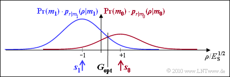
(5) With the decision boundary in the middle between the symbols ($G = 0$), the result is analogous to subtask (2) with the noise variance now larger:
- $$p_{\rm S} = {\rm Q} \left ( \frac{d/2}{\sigma_n} \right ) = {\rm Q} \left ( \frac{\sqrt{E_{\rm S}}}{\sqrt{E_{\rm S}}} \right )= {\rm Q} (1)\hspace{0.1cm} \hspace{0.15cm}\underline {\approx 15.9 \%} \hspace{0.05cm}.$$
The parameter $\gamma$ (normalized best possible displacement of the decision boundary) is
- $$\gamma = 2 \cdot \frac{ \sigma_n^2}{d^2} \cdot {\rm ln} \hspace{0.15cm} \frac{{\rm Pr}( m_1)}{{\rm Pr}( m_0)} = \frac{ 2 \cdot E_{\rm S}}{4 \cdot E_{\rm S}} \cdot {\rm ln} \hspace{0.15cm} \frac{2/3}{1/3} = \frac{{\rm ln} \hspace{0.15cm} 2}{2} \approx 0.35 $$
- $$\Rightarrow \hspace{0.3cm} G_{\rm opt} = 0.35 \cdot \sqrt{E_{\rm S}} \hspace{0.05cm}.$$
The more frequent symbol is now less frequently falsified ⇒ the mean error probability becomes smaller:
- $$p_{\rm S} = {2}/{3} \cdot {\rm Q} (1.35) + {1}/{3} \cdot {\rm Q} (0.65) = {2}/{3} \cdot 0.0885 +{1}/{3} \cdot 0.258 \hspace{0.1cm} \hspace{0.15cm}\underline {\approx 14.5 \%} \hspace{0.05cm}.$$
The figure makes it clear that the optimal decision boundary can also be determined graphically as the intersection of the two (weighted) probability density functions:
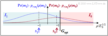
(6) All solutions of this rather academic subtask are correct:
- With threshold $G = 0$, we get $p_{\rm S} = {\rm Q}(0.5) \ \underline {\approx 0.309}$.
- The parameter $\gamma = 1.4$ now has four times the value compared to subtask (5),
so that the optimal decision boundary is now $G_{\rm opt} = \underline {1.4 \cdot s_0}$. - Thus, the (undisturbed) signal value $s_0$ does not belong to the decision region $I_0$, but to $I_1$, characterized by $\rho < G_{\rm opt}$.
- Only with a (positive) noise component $I_0 (\rho > G_{\rm opt})$ is possible at all. For the error probability, with $G_{\rm opt} = 1.4 \cdot s_0$:
- $$p_{\rm S} \hspace{-0.1cm} \ = \ \hspace{-0.1cm} {2}/{3} \cdot {\rm Q} (0.5 \cdot (1 + 1.4)) + {1}/{3} \cdot {\rm Q} (0.5 \cdot (1 - 1.4)) = \hspace{0.15cm}\underline {\approx 27\%} \hspace{0.05cm}.$$
The accompanying graph illustrates the statements made here.


