Difference between revisions of "Digital Signal Transmission/Binary Symmetric Channel"
| Line 8: | Line 8: | ||
== Binary Symmetric Channel – Model and Error Correlation Function== | == Binary Symmetric Channel – Model and Error Correlation Function== | ||
<br> | <br> | ||
| − | The left graph shows the BSC model, the simplest model of a digital transmission system. | + | The left graph shows the BSC model, the simplest model of a digital transmission system. |
| − | The name stands for '''Binary Symmetric Channel''' and states that this model can only be used for binary systems with symmetrical falsification properties. | + | The name stands for "'''Binary Symmetric Channel'''" and states that this model can only be used for binary systems with symmetrical falsification properties. |
[[File:EN_Dig_T_5_2_S1.png|right|frame|BSC model and associated error correlation function|class=fit]] | [[File:EN_Dig_T_5_2_S1.png|right|frame|BSC model and associated error correlation function|class=fit]] | ||
| − | *The BSC model is suitable for the study and generation of | + | Further applies: |
| − | + | *The BSC model is suitable for the study and generation of an error sequence with statistically independent errors. | |
| − | The right graph shows the | + | *Such a channel is also called "memory-free" and unlike the [[Digital_Signal_Transmission/Burst_Error_Channels|"burst error channel models"]] only a single channel state exists.<br> |
| + | |||
| + | *The two symbols $($for example $\rm L$ and $\rm H)$ are each falsified with the same probability $p$, so that the mean error probability $p_{\rm M} = p$ is also independent of the symbol probabilities $p_{\rm L}$ and $p_{\rm H}$.<br><br> | ||
| + | |||
| + | The right graph shows the "error correlation function" $\rm (ECF)$ of the BSC model: | ||
::<math>\varphi_{e}(k) = {\rm E}\big[e_{\nu} \cdot e_{\nu + k}\big] = | ::<math>\varphi_{e}(k) = {\rm E}\big[e_{\nu} \cdot e_{\nu + k}\big] = | ||
| Line 26: | Line 30: | ||
{{BlaueBox|TEXT= | {{BlaueBox|TEXT= | ||
$\text{Conclusion:}$ | $\text{Conclusion:}$ | ||
| − | *In the BSC model, the final ECF value (square of the mean error probability), which in other models is valid only for $k \to \infty$, is reached exactly at $k = 1$ and then remains constant.<br> | + | *In the BSC model, the final ECF value $($square of the mean error probability$)$, which in other models is valid only for $k \to \infty$, is reached exactly at $k = 1$ and then remains constant.<br> |
| − | *The BSC model belongs to the class of | + | *The BSC model belongs to the class of "renewal channel models". In a renewal channel model, the error distances are statistically independent of each other and the error correlation function can be calculated iteratively in a simple way: |
::<math>\varphi_{e}(k) = \sum_{\kappa = 1}^{k} {\rm Pr}(a = \kappa) \cdot | ::<math>\varphi_{e}(k) = \sum_{\kappa = 1}^{k} {\rm Pr}(a = \kappa) \cdot | ||
| Line 35: | Line 39: | ||
== Binary Symmetric Channel – Error Distance Distribution== | == Binary Symmetric Channel – Error Distance Distribution== | ||
<br> | <br> | ||
| − | We now consider the | + | We now consider the "error distance distribution" $\rm (EDD)$. The probability for the error distance $a=k$ is obtained from the condition of $k-1$ error-free symbols and one transmission error at time $\nu +k$, assuming that the last error occurred at time $\nu$. One obtains: |
::<math>{\rm Pr}(a = k) = (1-p)^{k-1}\cdot p \hspace{0.05cm}.</math> | ::<math>{\rm Pr}(a = k) = (1-p)^{k-1}\cdot p \hspace{0.05cm}.</math> | ||
It follows: | It follows: | ||
| − | *The error distance $a = 1$ always occurs with the greatest probability | + | *The error distance $a = 1$ always occurs in the BSC model with the greatest probability, and this for any value of $p$.<br> |
| − | *This fact is somewhat surprising at first glance | + | |
| − | + | *This fact is somewhat surprising at first glance: | |
| + | |||
| + | :With $p = 0.01$, for example, the mean error distance is ${\rm E}\big[a\big] = 100$. Nevertheless, two consecutive errors $(a = 1)$ are more probable by a factor of $0.99^{99} \approx 2.7$ than the error distance $a = 100$.<br><br> | ||
| − | The error distance distribution is obtained by summation according to the [[Digital_Signal_Transmission/Parameters_of_Digital_Channel_Models#Error_distance_distribution|"general definition"]]: | + | *The error distance distribution is obtained by summation according to the [[Digital_Signal_Transmission/Parameters_of_Digital_Channel_Models#Error_distance_distribution|"general definition"]]: |
::<math>V_a(k) = {\rm Pr}(a \ge k) = 1 - \sum_{\kappa = 1}^{k} (1-p)^{\kappa-1}\cdot p = (1-p)^{k-1}\hspace{0.05cm}.</math> | ::<math>V_a(k) = {\rm Pr}(a \ge k) = 1 - \sum_{\kappa = 1}^{k} (1-p)^{\kappa-1}\cdot p = (1-p)^{k-1}\hspace{0.05cm}.</math> | ||
| Line 56: | Line 62: | ||
| − | The decrease is exponential with increasing $k$ and is steeper the smaller $p$ is.<br> | + | ⇒ The decrease is exponential with increasing $k$ and is steeper the smaller $p$ is.<br> |
| − | The right graph shows the logarithmic representation. Here the drop is linear according to | + | ⇒ The right graph shows the logarithmic representation. Here the drop is linear according to |
::<math>{\rm lg} \hspace{0.15cm}V_a(k) = (k - 1) \cdot {\rm lg} \hspace{0.15cm}(1-p)\hspace{0.05cm}.</math>}}<br> | ::<math>{\rm lg} \hspace{0.15cm}V_a(k) = (k - 1) \cdot {\rm lg} \hspace{0.15cm}(1-p)\hspace{0.05cm}.</math>}}<br> | ||
| Line 64: | Line 70: | ||
== Applications of the BSC model == | == Applications of the BSC model == | ||
<br> | <br> | ||
| − | The BSC model is the | + | The BSC model is the "digital equivalent" of the simplest analog model ⇒ [[Digital_Signal_Transmission/Structure_of_the_Optimal_Receiver#Some_properties_of_the_AWGN_channel|"AWGN"]] for a time-invariant digital system corresponding to the following graph. It holds |
| + | [[File:P ID1830 Dig T 5 2 S3 version1.png|right|frame|On the use of the BSC model|class=fit]] | ||
| + | #The only degradation is noise. | ||
| + | #There is no distortion.<br> | ||
| + | |||
| + | |||
| + | To use the BSC model, the digital system must meet the following requirements: | ||
| + | *Redundancy-free binary encoding ⇒ no channel encoding and decoding,<br> | ||
| − | + | *noise according to the AWGN model ⇒ additive, white, Gaussian distributed,<br> | |
| + | |||
| + | *no distortions due to the components of the transmitter and receiver,<br> | ||
| − | |||
| − | |||
| − | |||
| − | |||
*threshold decision with symmetric decision threshold,<br> | *threshold decision with symmetric decision threshold,<br> | ||
| + | |||
*no extraneous influences such as crosstalk, dial pulses or electromagnetic interference fields.<br> | *no extraneous influences such as crosstalk, dial pulses or electromagnetic interference fields.<br> | ||
| − | + | ||
| + | |||
For a ''radio system'' with a direct line-of-sight between transmitter and receiver, the application of the BSC model is often justified, but not if fading influences ⇒ [[Digital_Signal_Transmission/Carrier_Frequency_Systems_with_Non-Coherent_Demodulation#Rayleigh_and_Rice_Distribution|"Rayleigh or Rice"]] play a role or if echoes may occur ⇒ [[Mobile_Communications/Multi-Path_Reception_in_Mobile_Communications|"multi-path reception"]].<br> | For a ''radio system'' with a direct line-of-sight between transmitter and receiver, the application of the BSC model is often justified, but not if fading influences ⇒ [[Digital_Signal_Transmission/Carrier_Frequency_Systems_with_Non-Coherent_Demodulation#Rayleigh_and_Rice_Distribution|"Rayleigh or Rice"]] play a role or if echoes may occur ⇒ [[Mobile_Communications/Multi-Path_Reception_in_Mobile_Communications|"multi-path reception"]].<br> | ||
Revision as of 13:07, 5 September 2022
Contents
Binary Symmetric Channel – Model and Error Correlation Function
The left graph shows the BSC model, the simplest model of a digital transmission system.
The name stands for "Binary Symmetric Channel" and states that this model can only be used for binary systems with symmetrical falsification properties.
Further applies:
- The BSC model is suitable for the study and generation of an error sequence with statistically independent errors.
- Such a channel is also called "memory-free" and unlike the "burst error channel models" only a single channel state exists.
- The two symbols $($for example $\rm L$ and $\rm H)$ are each falsified with the same probability $p$, so that the mean error probability $p_{\rm M} = p$ is also independent of the symbol probabilities $p_{\rm L}$ and $p_{\rm H}$.
The right graph shows the "error correlation function" $\rm (ECF)$ of the BSC model:
- \[\varphi_{e}(k) = {\rm E}\big[e_{\nu} \cdot e_{\nu + k}\big] = \left\{ \begin{array}{c} p \\ p^2 \end{array} \right.\quad \begin{array}{*{1}c} f{\rm or }\hspace{0.25cm}k = 0 \hspace{0.05cm}, \\ f{\rm or }\hspace{0.25cm} k > 0 \hspace{0.05cm}.\\ \end{array}\]
$\text{Conclusion:}$
- In the BSC model, the final ECF value $($square of the mean error probability$)$, which in other models is valid only for $k \to \infty$, is reached exactly at $k = 1$ and then remains constant.
- The BSC model belongs to the class of "renewal channel models". In a renewal channel model, the error distances are statistically independent of each other and the error correlation function can be calculated iteratively in a simple way:
- \[\varphi_{e}(k) = \sum_{\kappa = 1}^{k} {\rm Pr}(a = \kappa) \cdot \varphi_{e}(k - \kappa) \hspace{0.05cm}.\]
Binary Symmetric Channel – Error Distance Distribution
We now consider the "error distance distribution" $\rm (EDD)$. The probability for the error distance $a=k$ is obtained from the condition of $k-1$ error-free symbols and one transmission error at time $\nu +k$, assuming that the last error occurred at time $\nu$. One obtains:
- \[{\rm Pr}(a = k) = (1-p)^{k-1}\cdot p \hspace{0.05cm}.\]
It follows:
- The error distance $a = 1$ always occurs in the BSC model with the greatest probability, and this for any value of $p$.
- This fact is somewhat surprising at first glance:
- With $p = 0.01$, for example, the mean error distance is ${\rm E}\big[a\big] = 100$. Nevertheless, two consecutive errors $(a = 1)$ are more probable by a factor of $0.99^{99} \approx 2.7$ than the error distance $a = 100$.
- The error distance distribution is obtained by summation according to the "general definition":
- \[V_a(k) = {\rm Pr}(a \ge k) = 1 - \sum_{\kappa = 1}^{k} (1-p)^{\kappa-1}\cdot p = (1-p)^{k-1}\hspace{0.05cm}.\]
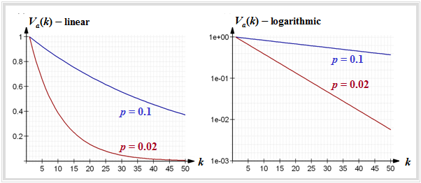
$\text{Example 1:}$ The left graph shows $V_a(k)$ in linear representation for
- $p = 0.1$ (blue curve), and
- $p = 0.02$ (red curve).
⇒ The decrease is exponential with increasing $k$ and is steeper the smaller $p$ is.
⇒ The right graph shows the logarithmic representation. Here the drop is linear according to
- \[{\rm lg} \hspace{0.15cm}V_a(k) = (k - 1) \cdot {\rm lg} \hspace{0.15cm}(1-p)\hspace{0.05cm}.\]
Applications of the BSC model
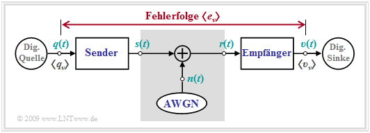
The BSC model is the "digital equivalent" of the simplest analog model ⇒ "AWGN" for a time-invariant digital system corresponding to the following graph. It holds
- The only degradation is noise.
- There is no distortion.
To use the BSC model, the digital system must meet the following requirements:
- Redundancy-free binary encoding ⇒ no channel encoding and decoding,
- noise according to the AWGN model ⇒ additive, white, Gaussian distributed,
- no distortions due to the components of the transmitter and receiver,
- threshold decision with symmetric decision threshold,
- no extraneous influences such as crosstalk, dial pulses or electromagnetic interference fields.
For a radio system with a direct line-of-sight between transmitter and receiver, the application of the BSC model is often justified, but not if fading influences ⇒ "Rayleigh or Rice" play a role or if echoes may occur ⇒ "multi-path reception".
In contrast, according to network operators, statistically independent errors tend to be the exception in the case of wireline transmission (for example, "DSL", but also optical transmission). If errors occur during data transmission via the telephone network, they are usually clustered.
In this case, we speak of so-called burst errors, which will be discussed in the next chapter.
Exercises for the chapter
Exercise 5.3: AWGN and BSC Model
Exercise 5.3Z: Analysis of the BSC Model
Exercise 5.4: Is the BSC Model Renewing?
Exercise 5.5: Error Sequence and Error Distance Sequence


