Difference between revisions of "Information Theory/Differential Entropy"
| Line 414: | Line 414: | ||
\int_{-\infty}^{+\infty}\hspace{-0.1cm} x^2 \cdot f_X(x) \hspace{0.1cm}{\rm d}x \hspace{0.05cm}.$$ | \int_{-\infty}^{+\infty}\hspace{-0.1cm} x^2 \cdot f_X(x) \hspace{0.1cm}{\rm d}x \hspace{0.05cm}.$$ | ||
| − | Following a similar procedure as in the [[Information_Theory/Differentielle_Entropie# | + | Following a similar procedure as in the [[Information_Theory/Differentielle_Entropie#Proof:_Maximum_differential_entropy_with_peak_constraint|proof of the peak constraint]] it turns out, that the „best possible” function $g_X(x) \sim {\rm e}^{–λ_2\hspace{0.05cm} · \hspace{0.05cm} x^2}$ must be ⇒ [[Theory_of_Stochastic_Signals/Gaußverteilte_Zufallsgröße|Gaussian distribution]]: |
:$$g_X(x) ={1}/{\sqrt{2\pi \sigma^2}} \cdot {\rm e}^{ | :$$g_X(x) ={1}/{\sqrt{2\pi \sigma^2}} \cdot {\rm e}^{ | ||
- \hspace{0.05cm}{x^2}/{(2 \sigma^2)} }\hspace{0.05cm}.$$ | - \hspace{0.05cm}{x^2}/{(2 \sigma^2)} }\hspace{0.05cm}.$$ | ||
| − | + | However, we use here for the explicit proof the [[Information_Theory/Einige_Vorbemerkungen_zu_zweidimensionalen_Zufallsgrößen#Informational_Divergence_-_Kullback-Leibler_Distance|Kullback–Leibler distance]] between a suitable general PDF $f_X(x)$ and the Gaussian PDF $g_X(x)$: | |
:$$D(f_X \hspace{0.05cm} || \hspace{0.05cm}g_X) = \int_{-\infty}^{+\infty} \hspace{0.02cm} | :$$D(f_X \hspace{0.05cm} || \hspace{0.05cm}g_X) = \int_{-\infty}^{+\infty} \hspace{0.02cm} | ||
| Line 426: | Line 426: | ||
f_X(x) \cdot {\rm ln} \hspace{0.1cm} {g_X(x)} \hspace{0.1cm}{\rm d}x \hspace{0.05cm}.$$ | f_X(x) \cdot {\rm ln} \hspace{0.1cm} {g_X(x)} \hspace{0.1cm}{\rm d}x \hspace{0.05cm}.$$ | ||
| − | + | For simplicity, the natural logarithm ⇒ $\ln$ is used here. Thus we obtain for the second integral: | |
:$$I_2 = - \frac{1}{2} \cdot {\rm ln} \hspace{0.1cm} (2\pi\sigma^2) \cdot \hspace{-0.1cm}\int_{-\infty}^{+\infty} \hspace{-0.4cm} f_X(x) \hspace{0.1cm}{\rm d}x | :$$I_2 = - \frac{1}{2} \cdot {\rm ln} \hspace{0.1cm} (2\pi\sigma^2) \cdot \hspace{-0.1cm}\int_{-\infty}^{+\infty} \hspace{-0.4cm} f_X(x) \hspace{0.1cm}{\rm d}x | ||
| Line 433: | Line 433: | ||
\hspace{0.05cm}.$$ | \hspace{0.05cm}.$$ | ||
| − | + | By definition, the first integral is equal to $1$ and the second integral gives $σ^2$: | |
:$$I_2 = - {1}/{2} \cdot {\rm ln} \hspace{0.1cm} (2\pi\sigma^2) - {1}/{2} \cdot [{\rm ln} \hspace{0.1cm} ({\rm e})] = - {1}/{2} \cdot {\rm ln} \hspace{0.1cm} (2\pi{\rm e} \cdot \sigma^2)$$ | :$$I_2 = - {1}/{2} \cdot {\rm ln} \hspace{0.1cm} (2\pi\sigma^2) - {1}/{2} \cdot [{\rm ln} \hspace{0.1cm} ({\rm e})] = - {1}/{2} \cdot {\rm ln} \hspace{0.1cm} (2\pi{\rm e} \cdot \sigma^2)$$ | ||
| Line 439: | Line 439: | ||
-h(X) + {1}/{2} \cdot {\rm ln} \hspace{0.1cm} (2\pi{\rm e} \cdot \sigma^2)\hspace{0.05cm}.$$ | -h(X) + {1}/{2} \cdot {\rm ln} \hspace{0.1cm} (2\pi{\rm e} \cdot \sigma^2)\hspace{0.05cm}.$$ | ||
| − | + | Since also for continuous value random variables the Kullback-Leibler distance is always $\ge 0$ , after generalisation („ln” ⇒ „log”): | |
:$$h(X) \le {1}/{2} \cdot {\rm log} \hspace{0.1cm} (2\pi{\rm e} \cdot \sigma^2)\hspace{0.05cm}.$$ | :$$h(X) \le {1}/{2} \cdot {\rm log} \hspace{0.1cm} (2\pi{\rm e} \cdot \sigma^2)\hspace{0.05cm}.$$ | ||
| − | + | The equal sign only applies if the random variable $X$ Gaussian distributed. | |
{{BlaueBox|TEXT= | {{BlaueBox|TEXT= | ||
| − | $\text{ | + | $\text{Summary for power constraints:}$ |
| − | + | The maximum differential entropy is obtained under the condition ${\rm E}\big[ \vert X – m_1 \vert ^2 \big] ≤ σ^2$ independent of $m_1$ for the '''Gaussian PDF''': | |
:$$h_{\rm max}(X) = {1}/{2} \cdot {\rm log} \hspace{0.1cm} ({\it \Gamma}_{\hspace{-0.01cm} \rm L} \cdot \sigma^2) = | :$$h_{\rm max}(X) = {1}/{2} \cdot {\rm log} \hspace{0.1cm} ({\it \Gamma}_{\hspace{-0.01cm} \rm L} \cdot \sigma^2) = | ||
{1}/{2} \cdot {\rm log} \hspace{0.1cm} (2\pi{\rm e} \cdot \sigma^2) \hspace{0.5cm} \Rightarrow\hspace{0.5cm} {\it \Gamma}_{\rm L} = 2\pi{\rm e} | {1}/{2} \cdot {\rm log} \hspace{0.1cm} (2\pi{\rm e} \cdot \sigma^2) \hspace{0.5cm} \Rightarrow\hspace{0.5cm} {\it \Gamma}_{\rm L} = 2\pi{\rm e} | ||
\hspace{0.05cm}.$$ | \hspace{0.05cm}.$$ | ||
| − | + | Any other continuous value random variable $X$ with variance ${\rm E}\big[ \vert X – m_1 \vert ^2 \big] ≤ σ^2$ leads to a smaller value, characterised by the parameter ${\it \Gamma}_{\rm L} < 2πe$. }} | |
| − | == | + | ==Relevant tasks== |
<br> | <br> | ||
[[Aufgaben:4.1 WDF, VTF und Wahrscheinlichkeit|Aufgabe 4.1: WDF, VTF und Wahrscheinlichkeit]] | [[Aufgaben:4.1 WDF, VTF und Wahrscheinlichkeit|Aufgabe 4.1: WDF, VTF und Wahrscheinlichkeit]] | ||
Revision as of 14:16, 15 April 2021
Contents
- 1 # OVERVIEW OF THE FOURTH MAIN CHAPTER #
- 2 Properties of continuous-value random variables
- 3 Entropy of continuous-value random variables after quantisation
- 4 Definition and properties of differential entropy
- 5 Differential entropy of some peak-constrained random variables
- 6 Differential entropy of some power-constrained random variables
- 7 Proof: Maximum differential entropy with peak constraint
- 8 Proof: Maximum differential entropy with power constraint
- 9 Relevant tasks
# OVERVIEW OF THE FOURTH MAIN CHAPTER #
In the last chapter of this book, the information-theoretical quantities defined so far for the discrete-value case are adapted in such a way that they can also be applied to continuous-value random quantities.
- For example, the entropy $H(X)$ for the discrete-value random variable $X$ becomes the differential entropy $h(X)$ in the continuous-value case.
- While $H(X)$ indicates the „uncertainty” with regard to the discrete random variable $X$ with regard to the discrete random variable $h(X)$ in the same way in the continuous case.
Many of the relationships derived in the third chapter „Information between two discrete-value random variables ⇒ see table of contents for conventional entropy also apply to differential entropy. Thus, the differential joint entropy $h(XY)$ can also be given for continuous-value random variables $X$ and $Y$ and likewise the two conditional differential entropies $h(Y|X)$ and $h(X|Y)$.
In detail, this main chapter deals with:
- the special features of continuous value random variables,
- the definition and calculation of the differential entropy as well as its properties,
- the mutual information between two value-continuous random variables,
- the capacity of the AWGN channel and several such parallel Gaussian channels,
- the channel coding theorem, one of the „highlights” of Shannon's information theory,
- the AWGN channel capacity for discrete-value input sines (BPSK, QPSK).
Properties of continuous-value random variables
Up to now, discrete-value random variables of the form $X = \{x_1,\ x_2, \hspace{0.05cm}\text{...}\hspace{0.05cm} , x_μ, \text{...} ,\ x_M\}$ have always been considered, which from an information-theoretical point of view are completely characterised by their probability mass function (PMF) $P_X(X)$ :
- $$P_X(X) = \big [ \hspace{0.1cm} p_1, p_2, \hspace{0.05cm}\text{...} \hspace{0.15cm}, p_{\mu},\hspace{0.05cm} \text{...}\hspace{0.15cm}, p_M \hspace{0.1cm}\big ] \hspace{0.3cm}{\rm mit} \hspace{0.3cm} p_{\mu}= P_X(x_{\mu})= {\rm Pr}( X = x_{\mu}) \hspace{0.05cm}.$$
A continuous-value random variable, ' on the other hand, can assume any value – at least in finite intervals:
- Due to the uncountable supply of values, the description by a probability function is not possible in this case, or at least it does not make sense:
- This would result in $M \to ∞$ as well as $p_1 \to 0$, $p_2 \to 0$, etc.
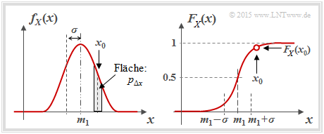
For the description of value-continuous random variables, one uses equally according to the definitions in the book Theory of Stochastic Signals :
- the probability density function (PDF):
- $$f_X(x_0)= \lim_{{\rm \Delta} x\to \rm 0}\frac{p_{{\rm \Delta} x}}{{\rm \Delta} x} = \lim_{{\rm \Delta} x\to \rm 0}\frac{{\rm Pr} \{ x_0- {\rm \Delta} x/\rm 2 \le \it X \le x_{\rm 0} +{\rm \Delta} x/\rm 2\}}{{\rm \Delta} x};$$
- In words: the PDF value at $x_0$ gives the probability $p_{Δx}$ that $X$ lies in an (infinitely small) interval of width $Δx$ around $x_0$ , divided by $Δx$; (note the entries in the adjacent graph);
- the mean value (first moment):
- $$m_1 = {\rm E}\big[ X \big]= \int_{-\infty}^{+\infty} \hspace{-0.1cm} x \cdot f_X(x) \hspace{0.1cm}{\rm d}x \hspace{0.05cm};$$
- the variance (second moment):
- $$\sigma^2 = {\rm E}\big[(X- m_1 )^2 \big]= \int_{-\infty}^{+\infty} \hspace{-0.1cm} (x- m_1 )^2 \cdot f_X(x- m_1 ) \hspace{0.1cm}{\rm d}x \hspace{0.05cm};$$
- the cumulative distribution fucntion (CDF):
- $$F_X(x) = \int_{-\infty}^{x} \hspace{-0.1cm}f_X(\xi) \hspace{0.1cm}{\rm d}\xi \hspace{0.2cm} = \hspace{0.2cm} {\rm Pr}(X \le x)\hspace{0.05cm}.$$
Note that both the PDF area and the CDF final value are always equal to $1$ .
$\text{Nomenclature notes on PDF and CDF:}$
We use in this chapter for a probability density function the representation form $f_X(x)$ often used in the literature, where holds::
- $X$ denotes the (discrete-value or continuous-value) random variable,
- $x$ is a possible realisation of $X$ ⇒ $x ∈ X$.
Accordingly, we denote the cumulative distribution function (CDF) of the random variable $X$ by $F_X(x)$ according to the following definition:
- $$F_X(x) = \int_{-\infty}^{x} \hspace{-0.1cm}f_X(\xi) \hspace{0.1cm}{\rm d}\xi \hspace{0.2cm} = \hspace{0.2cm} {\rm Pr}(X \le x)\hspace{0.05cm}.$$
In other $\rm LNTwww$ books, we often write so as not to use up two characters for one variable:
- For the PDF $f_x(x)$ ⇒ no distinction between random variable and realising, and
- for the CDF $F_x(r) = {\rm Pr}(x ≤ r)$ ⇒ here one needs a second variable in any case.
We apologise for this formal inaccuracy.
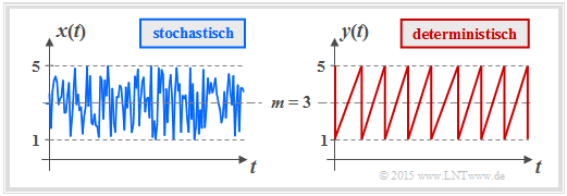
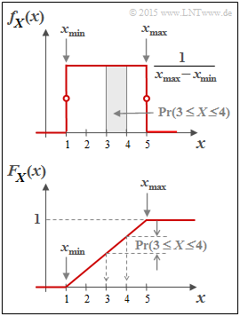
$\text{Example 1:}$ We now consider an important special case with the uniform distribution.
- The graph shows the course of two uniformly distributed variables, which can assume all values between $1$ and $5$ $($mean value $m_1 = 3)$ with equal probability.
- On the left is the result of a random process, on the right a deterministic signal with the same amplitude distribution.
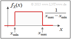
The probability density function of the uniform distribution has the course sketched in the second graph above:
- $$f_X(x) = \left\{ \begin{array}{c} \hspace{0.25cm}(x_{\rm max} - x_{\rm min})^{-1} \\ 1/2 \cdot (x_{\rm max} - x_{\rm min})^{-1} \\ \hspace{0.25cm} 0 \\ \end{array} \right. \begin{array}{*{20}c} {\rm{f\ddot{u}r} } \\ {\rm{f\ddot{u}r} } \\ {\rm{f\ddot{u}r} } \\ \end{array} \begin{array}{*{20}l} {x_{\rm min} < x < x_{\rm max},} \\ x ={x_{\rm min} \hspace{0.1cm}{\rm und}\hspace{0.1cm}x = x_{\rm max},} \\ x > x_{\rm max}. \\ \end{array}$$
The following equations are obtained here for the mean $m_1 ={\rm E}\big[X\big]$ and the variance $σ^2={\rm E}\big[(X – m_1)^2\big]$ :
- $$m_1 = \frac{x_{\rm max} + x_{\rm min} }{2}\hspace{0.05cm}, $$
- $$\sigma^2 = \frac{(x_{\rm max} - x_{\rm min})^2}{12}\hspace{0.05cm}.$$
Shown below is the cumulative distribution function (CDF):
- $$F_X(x) = \int_{-\infty}^{x} \hspace{-0.1cm}f_X(\xi) \hspace{0.1cm}{\rm d}\xi \hspace{0.2cm} = \hspace{0.2cm} {\rm Pr}(X \le x)\hspace{0.05cm}.$$
- This is identically zero for $x ≤ x_{\rm min}$, increases linearly thereafter and reaches the CDF final value of $1$ at $x = x_{\rm max}$ .
- The probability that the random variable $X$ takes on a value between $3$ and $4$ can be determined from both the PDF and the CDF:
- $${\rm Pr}(3 \le X \le 4) = \int_{3}^{4} \hspace{-0.1cm}f_X(\xi) \hspace{0.1cm}{\rm d}\xi = 0.25\hspace{0.05cm}\hspace{0.05cm},$$
- $${\rm Pr}(3 \le X \le 4) = F_X(4) - F_X(3) = 0.25\hspace{0.05cm}.$$
Furthermore, note:
- The result $X = 0$ is excluded for this random variable ⇒ ${\rm Pr}(X = 0) = 0$.
- The result $X = 4$ , on the other hand, is quite possible. Nevertheless, auch hier ${\rm Pr}(X = 4) = 0 $also applies here.
Entropy of continuous-value random variables after quantisation
We now consider a continuous value random variable $X$ in the range $0 \le x \le 1$.
- We quantise the continuous random variable $X$, in order to be able to further apply the previous entropy calculation. We call the resulting discrete (quantised) quantity $Z$.
- Let the number of quantisation steps be $M$, so that each quantisation interval $μ$ has the width ${\it Δ} = 1/M$ in the present PDF. We denote the interval centres by $x_μ$.
- The probability $p_μ = {\rm Pr}(Z = z_μ)$ with respect to $Z$ is equal to the probability that the continuous random variable $X$ has a value between $x_μ - {\it Δ}/2$ and $x_μ + {\it Δ}/2$ .
- First we set $M = 2$ and then double this value in each iteration. This makes the quantisation increasingly finer. In the $n$th try gilt dann $M = 2^n$ and ${\it Δ} =2^{–n}$ then apply.
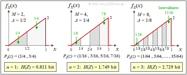
$\text{Example 2:}$ The graph shows the results of the first three trials for an asymmetrical triangular PDF $($betweeen $0$ and $1)$:
- $n = 1 \ ⇒ \ M = 2 \ ⇒ \ {\it Δ} = 1/2\text{:}$ $H(Z) = 0.811\ \rm bit,$
- $n = 2 \ ⇒ \ M = 4 \ ⇒ \ {\it Δ} = 1/4\text{:}$ $H(Z) = 1.749\ \rm bit,$
- $n = 3 \ ⇒ \ M = 8 \ ⇒ \ {\it Δ} = 1/8\text{:}$ $H(Z) = 2.729\ \rm bit.$
Additionally, the following quantities can be taken from the graph, for example for ${\it Δ} = 1/8$:
- The interval centres are at
- $$x_1 = 1/16,\ x_2 = 3/16,\text{ ...} \ ,\ x_8 = 15/16 $$
- $$ ⇒ \ x_μ = {\it Δ} · (μ - 1/2).$$
- The interval areas result in
- $$p_μ = {\it Δ} · f_X(x_μ) ⇒ p_8 = 1/8 · (7/8+1)/2 = 15/64.$$
- Thus, for the probability function of the quantised random variabl $Z$, we obtain::
- $$P_Z(Z) = (1/64, \ 3/64, \ 5/64, \ 7/64, \ 9/64, \ 11/64, \ 13/64, \ 15/64).$$
$\text{Conclusion:}$ We interpret the results of this experiment as follows:
- The entropy $H(Z)$ becomes larger and larger as $M$ increases.
- The limit of $H(Z)$ for $M \to ∞ \ ⇒ \ {\it Δ} → 0$ is infinite.
- Thus, the entropy $H(X)$ of the continuous-value random variable $X$ is also infinite.
- It follows: The previous definition of entropy fails here.
To verify our empirical result, we assume the following equation:
- $$H(Z) = \hspace{0.2cm} \sum_{\mu = 1}^{M} \hspace{0.2cm} p_{\mu} \cdot {\rm log}_2 \hspace{0.1cm} \frac{1}{p_{\mu}}= \hspace{0.2cm} \sum_{\mu = 1}^{M} \hspace{0.2cm} {\it \Delta} \cdot f_X(x_{\mu} ) \cdot {\rm log}_2 \hspace{0.1cm} \frac{1}{{\it \Delta} \cdot f_X(x_{\mu} )}\hspace{0.05cm}.$$
We now split $H(Z) = S_1 + S_2$ into two sums:
- $$\begin{align*}S_1 & = {\rm log}_2 \hspace{0.1cm} \frac{1}{\it \Delta} \cdot \hspace{0.2cm} \sum_{\mu = 1}^{M} \hspace{0.02cm} {\it \Delta} \cdot f_X(x_{\mu} ) \approx - {\rm log}_2 \hspace{0.1cm}{\it \Delta} \hspace{0.05cm},\\ S_2 & = \hspace{0.05cm} \sum_{\mu = 1}^{M} \hspace{0.2cm} f_X(x_{\mu} ) \cdot {\rm log}_2 \hspace{0.1cm} \frac{1}{ f_X(x_{\mu} ) } \cdot {\it \Delta} \hspace{0.2cm}\approx \hspace{0.2cm} \int_{0}^{1} \hspace{0.05cm} f_X(x) \cdot {\rm log}_2 \hspace{0.1cm} \frac{1}{ f_X(x) } \hspace{0.1cm}{\rm d}x \hspace{0.05cm}.\end{align*}$$
- The approximation $S_1 ≈ -\log_2 {\it Δ}$ applies exactly only in the borderline case ${\it Δ} → 0$.
- The given approximation for $S_2$ is also only valid for small ${\it Δ} → {\rm d}x$, so that one should replace the sum by the integral.
$\text{Generalisation:}$ If one approximates the value-continuous random variable $X$ with the PDF $f_X(x)$ by a discrete-value random variable $Z$ by performing a (fine) quantisation with the interval width ${\it Δ}$ , one obtains for the entropy of the random variable $Z$:
- $$H(Z) \approx - {\rm log}_2 \hspace{0.1cm}{\it \Delta} \hspace{0.2cm}+ \hspace{-0.35cm} \int\limits_{\text{supp}(f_X)} \hspace{-0.35cm} f_X(x) \cdot {\rm log}_2 \hspace{0.1cm} \frac{1}{ f_X(x) } \hspace{0.1cm}{\rm d}x = - {\rm log}_2 \hspace{0.1cm}{\it \Delta} \hspace{0.2cm} + h(X) \hspace{0.5cm}\big [{\rm in \hspace{0.15cm}bit}\big ] \hspace{0.05cm}.$$
The integral describes the differential entropy $h(X)$ of the continuous-value random variable $X$. For the special case ${\it Δ} = 1/M = 2^{-n}$ , the above equation can also be written as follows:
- $$H(Z) = n + h(X) \hspace{0.5cm}\big [{\rm in \hspace{0.15cm}bit}\big ] \hspace{0.05cm}.$$
- In the borderline case ${\it Δ} → 0 \ ⇒ \ M → ∞ \ ⇒ \ n → ∞$ , the entropy of the continuous-value random variable is also infinite: $H(X) → ∞$.
- Even with smaller $n$ , this equation is only an approximation for $H(Z)$ , with the differential entropy $h(X)$ of the continuous-value quantity serving as a correction factor.
$\text{Example 3:}$ As in $\text{example 2}$ , we consider a triangular PDF $($between $0$ and $1)$. Its differential entropy, as calculated in task 4.2 results in
- $$h(X) = \hspace{0.05cm}-0.279 \ \rm bit.$$
- The table shows the entropy $H(Z)$ of the quantity $Z$ quantised with $n$ bits .
- Already fo $n = 3$ one can see an agreement between the approximation (lower row) and the exact calculation (row 2).
- For $n = 10$ , the approximation will agree even better with the exact calculation (which is extremely time-consuming) .
Definition and properties of differential entropy
$\text{Generalisation:}$ The differential entropy $h(X)$ of a continuous value random variable $X$ with probability density function $f_X(x)$ is:
- $$h(X) = \hspace{0.1cm} - \hspace{-0.45cm} \int\limits_{\text{supp}(f_X)} \hspace{-0.35cm} f_X(x) \cdot {\rm log} \hspace{0.1cm} \big[ f_X(x) \big] \hspace{0.1cm}{\rm d}x \hspace{0.6cm}{\rm mit}\hspace{0.6cm} {\rm supp}(f_X) = \{ x\text{:} \ f_X(x) > 0 \} \hspace{0.05cm}.$$
A pseudo-unit must be added in each case:
- „nat” when using „ln” ⇒ natural logarithm,
- „bit” when using „log2” ⇒ binary logarithm.
While the (conventional) entropy of a discrete-value random variable $X$ is always $H(X) ≥ 0$ , the differential entropy $h(X)$ of a continuous-value random variable can also be negative. From this it is already evident that $h(X)$ , in contrast to $H(X)$ , cannot be interpreted as „uncertainty”.
$\text{Example 4:}$ The upper graph shows the probability density of a random variable $X$ equally distributed between $x_{\rm min}$ and $x_{\rm max}$ . For its differential entropy one obtains in „nat”:
- $$\begin{align*}h(X) & = - \hspace{-0.18cm}\int\limits_{x_{\rm min} }^{x_{\rm max} } \hspace{-0.28cm} \frac{1}{x_{\rm max}\hspace{-0.05cm} - \hspace{-0.05cm}x_{\rm min} } \cdot {\rm ln} \hspace{0.1cm}\big [ \frac{1}{x_{\rm max}\hspace{-0.05cm} - \hspace{-0.05cm}x_{\rm min} }\big ] \hspace{0.1cm}{\rm d}x \\ & = {\rm ln} \hspace{0.1cm} \big[ {x_{\rm max}\hspace{-0.05cm} - \hspace{-0.05cm}x_{\rm min} }\big ] \cdot \big [ \frac{1}{x_{\rm max}\hspace{-0.05cm} - \hspace{-0.05cm}x_{\rm min} } \big ]_{x_{\rm min} }^{x_{\rm max} }={\rm ln} \hspace{0.1cm} \big[ {x_{\rm max}\hspace{-0.05cm} - \hspace{-0.05cm}x_{\rm min} } \big]\hspace{0.05cm}.\end{align*} $$
The equation for the differential entropy in „bit” is:
- $$h(X) = \log_2 \big[x_{\rm max} – x_{ \rm min} \big].$$
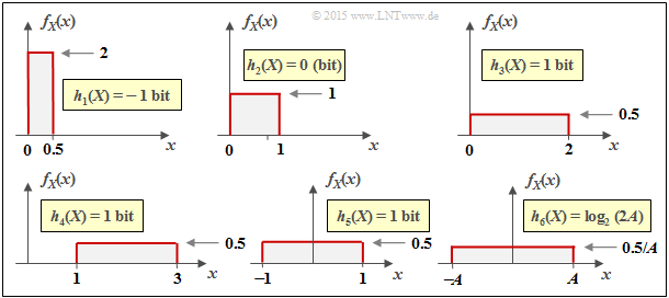
The graph on the left shows the numerical evaluation of the above result by means of some examples.
$\text{Interpretation:}$ From the six sketches in the last example, important properties of the differential entropy $h(X)$ can be read:
- The differential entropy is not changed by a PDF shift $($um $k)$ :
- $$h(X + k) = h(X) \hspace{0.2cm}\Rightarrow \hspace{0.2cm} \text{For example} \ \ h_3(X) = h_4(X) = h_5(X) \hspace{0.05cm}.$$
- $h(X)$ changes by compression/spreading of the PDF by the factor $k ≠ 0$ as follows:
- $$h( k\hspace{-0.05cm} \cdot \hspace{-0.05cm}X) = h(X) + {\rm log}_2 \hspace{0.05cm} \vert k \vert \hspace{0.2cm}\Rightarrow \hspace{0.2cm} \text{Beispielsweise gilt} \ \ h_6(X) = h_5(AX) = h_5(X) + {\rm log}_2 \hspace{0.05cm} (A) = {\rm log}_2 \hspace{0.05cm} (2A) \hspace{0.05cm}.$$
Furthermore, many of the equations derived in the chapter different entropies of two-dimensional Random Variables for the discrete-value case also apply to continuous-value random variables.
From the following compilation one can see that often only the (large) $H$ has to be replaced by a (small) $h$ as well as the probability mass function $\rm (PMF)$ by the corresponding probability density function $\rm (PDF)$ .
- Conditional Differential Entropy:
- $$H(X \hspace{-0.05cm}\mid \hspace{-0.05cm} Y) = {\rm E} \hspace{-0.1cm}\left [ {\rm log} \hspace{0.1cm}\frac{1}{P_{\hspace{0.03cm}X \mid \hspace{0.03cm} Y} (X \hspace{-0.05cm}\mid \hspace{-0.05cm} Y)}\right ]=\hspace{-0.04cm} \sum_{(x, y) \hspace{0.1cm}\in \hspace{0.1cm}{\rm supp} \hspace{0.03cm}(\hspace{-0.03cm}P_{XY}\hspace{-0.08cm})} \hspace{-0.8cm} P_{XY}(x, y) \cdot {\rm log} \hspace{0.1cm} \frac{1}{P_{\hspace{0.03cm}X \mid \hspace{0.03cm} Y} (x \hspace{-0.05cm}\mid \hspace{-0.05cm} y)} \hspace{0.05cm}$$
- $$\Rightarrow \hspace{0.3cm}h(X \hspace{-0.05cm}\mid \hspace{-0.05cm} Y) = {\rm E} \hspace{-0.1cm}\left [ {\rm log} \hspace{0.1cm}\frac{1}{f_{\hspace{0.03cm}X \mid \hspace{0.03cm} Y} (X \hspace{-0.05cm}\mid \hspace{-0.05cm} Y)}\right ]=\hspace{0.2cm} \int \hspace{-0.9cm} \int\limits_{\hspace{-0.04cm}(x, y) \hspace{0.1cm}\in \hspace{0.1cm}{\rm supp}\hspace{0.03cm}(\hspace{-0.03cm}f_{XY}\hspace{-0.08cm})} \hspace{-0.6cm} f_{XY}(x, y) \cdot {\rm log} \hspace{0.1cm} \frac{1}{f_{\hspace{0.03cm}X \mid \hspace{0.03cm} Y} (x \hspace{-0.05cm}\mid \hspace{-0.05cm} y)} \hspace{0.15cm}{\rm d}x\hspace{0.15cm}{\rm d}y\hspace{0.05cm}.$$
- Joint Differential Entropy:
- $$H(XY) = {\rm E} \left [ {\rm log} \hspace{0.1cm} \frac{1}{P_{XY}(X, Y)}\right ] =\hspace{-0.04cm} \sum_{(x, y) \hspace{0.1cm}\in \hspace{0.1cm}{\rm supp} \hspace{0.03cm}(\hspace{-0.03cm}P_{XY}\hspace{-0.08cm})} \hspace{-0.8cm} P_{XY}(x, y) \cdot {\rm log} \hspace{0.1cm} \frac{1}{ P_{XY}(x, y)} \hspace{0.05cm}$$
- $$\Rightarrow \hspace{0.3cm}h(XY) = {\rm E} \left [ {\rm log} \hspace{0.1cm} \frac{1}{f_{XY}(X, Y)}\right ] =\hspace{0.2cm} \int \hspace{-0.9cm} \int\limits_{\hspace{-0.04cm}(x, y) \hspace{0.1cm}\in \hspace{0.1cm}{\rm supp} \hspace{0.03cm}(\hspace{-0.03cm}f_{XY}\hspace{-0.08cm})} \hspace{-0.6cm} f_{XY}(x, y) \cdot {\rm log} \hspace{0.1cm} \frac{1}{ f_{XY}(x, y) } \hspace{0.15cm}{\rm d}x\hspace{0.15cm}{\rm d}y\hspace{0.05cm}.$$
- Chain rule of differential entropy:
- $$H(X_1\hspace{0.05cm}X_2\hspace{0.05cm}\text{...} \hspace{0.1cm}X_n) =\sum_{i = 1}^{n} H(X_i | X_1\hspace{0.05cm}X_2\hspace{0.05cm}\text{...} \hspace{0.1cm}X_{i-1}) \le \sum_{i = 1}^{n} H(X_i) \hspace{0.05cm}$$
- $$\Rightarrow \hspace{0.3cm} h(X_1\hspace{0.05cm}X_2\hspace{0.05cm}\text{...} \hspace{0.1cm}X_n) =\sum_{i = 1}^{n} h(X_i | X_1\hspace{0.05cm}X_2\hspace{0.05cm}\text{...} \hspace{0.1cm}X_{i-1}) \le \sum_{i = 1}^{n} h(X_i) \hspace{0.05cm}.$$
- Kullback–Leibler distance between the random variables $X$ and $Y$:
- $$D(P_X \hspace{0.05cm} || \hspace{0.05cm}P_Y) = {\rm E} \left [ {\rm log} \hspace{0.1cm} \frac{P_X(X)}{P_Y(X)}\right ] \hspace{0.2cm}=\hspace{0.2cm} \sum_{x \hspace{0.1cm}\in \hspace{0.1cm}{\rm supp} \hspace{0.03cm}(\hspace{-0.03cm}P_{X})\hspace{-0.8cm}} P_X(x) \cdot {\rm log} \hspace{0.1cm} \frac{P_X(x)}{P_Y(x)} \ge 0$$
- $$\Rightarrow \hspace{0.3cm}D(f_X \hspace{0.05cm} || \hspace{0.05cm}f_Y) = {\rm E} \left [ {\rm log} \hspace{0.1cm} \frac{f_X(X)}{f_Y(X)}\right ] \hspace{0.2cm}= \hspace{-0.4cm}\int\limits_{x \hspace{0.1cm}\in \hspace{0.1cm}{\rm supp}\hspace{0.03cm}(\hspace{-0.03cm}f_{X}\hspace{-0.08cm})} \hspace{-0.4cm} f_X(x) \cdot {\rm log} \hspace{0.1cm} \frac{f_X(x)}{f_Y(x)} \hspace{0.15cm}{\rm d}x \ge 0 \hspace{0.05cm}.$$
Differential entropy of some peak-constrained random variables
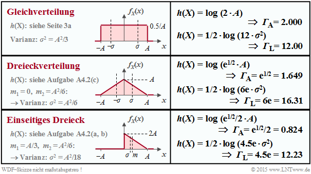
The table shows the results regarding the differential entropy for three exemplary probability density functions $f_X(x)$. These are all peak-constrained, i.e. $|X| ≤ A$ applies in each case.
- With peak constraint , the differential entropy can always be represented as follows:
- $$h(X) = {\rm log}\,\, ({\it \Gamma}_{\rm A} \cdot A).$$
The argument ${\it \Gamma}_A · A$ is independent of which logarithm one uses. To be added
- if $\ln$ is used, we use the pseudo-unit „nat”,
- if $\log_2$ is used, we use the pseudo-unit „bit”.
$\text{Theorem:}$ Under the peak contstraint ⇒ i.e. PDF $f_X(x) = 0$ for $ \vert x \vert > A$ – the uniform distribution leads to the maximum differential entropy:
- $$h_{\rm max}(X) = {\rm log} \hspace{0.1cm} (2A)\hspace{0.05cm}.$$
Here, the appropriate parameter ${\it \Gamma}_{\rm A} = 2$ is maximal. You will find the proof at the end of this chapter.
The theorem simultaneously means that for any other peak-constrained PDF (except the uniform distribution) the characteristic parameter ${\it \Gamma}_{\rm A} < 2$ .
- For the symmetric triangular distribution, the above table gives ${\it \Gamma}_{\rm A} = \sqrt{\rm e} ≈ 1.649$.
- In contrast, for the one-sided triangle $($between $0$ and $A)$ ${\it \Gamma}_{\rm A}$ is only half as large.
- For every other triangle $($width $A$, arbitrary peak between $0$ and $A)$ ${\it \Gamma}_{\rm A} ≈ 0.824$ also applies.
The respective second $h(X)$ specification and the characteristic ${\it \Gamma}_{\rm L}$ on the other hand, are suitable for the comparison of random variables with power constraints, which will be discussed in the next section. Under this constraint, for example, the symmetric triangular distribution $({\it \Gamma}_{\rm L} ≈ 16.31)$ is better than the uniform distribution ${\it \Gamma}_{\rm L} = 12)$.
Differential entropy of some power-constrained random variables
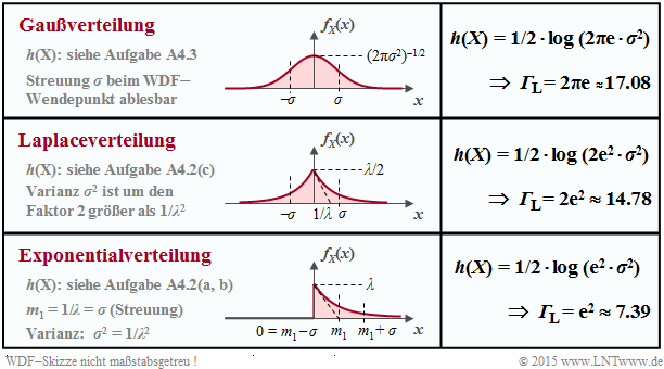
The differential entropies $h(X)$ for three exemplary density functions $f_X(x)$ without boundary, which all have the same variance $σ^2 = {\rm E}\big[|X -m_x|^2 \big]$ and thus the same dispersion $σ$ through appropriate parameter selection, can be taken from the following table. Considered are:
- the Gaussian distribution,
- the Laplace distribution ⇒ a two-sided exponential distribution,
- the (one-sided) exponential distribution.
The differential entropy can always be represented here as
- $$h(X) = 1/2 \cdot {\rm log} \hspace{0.1cm} ({\it \Gamma}_{\rm L} \cdot \sigma^2).$$
The result differs only by the pseudo-unit
- „nat” when using $\ln$ or
- „bit” when using $\log_2$.
$\text{Theorem:}$ Under the power constraint, the Gaussian distribution leads to
- $$f_X(x) = \frac{1}{\sqrt{2\pi \sigma^2} } \cdot {\rm exp} \left [ - \hspace{0.05cm}\frac{(x - m_1)^2}{2 \sigma^2}\right ]$$
independent of the mean $m_1$ to the maximum differential entropy:
- $$h(X) = 1/2 \cdot {\rm log} \hspace{0.1cm} (2\pi{\rm e} \cdot \sigma^2)\hspace{0.3cm}\Rightarrow\hspace{0.3cm}{\it \Gamma}_{\rm L} < 2π{\rm e} ≈ 17.08\hspace{0.05cm}.$$
You will find the proof at the end of this chapter.
This statement means at the same time that for any PDF other than the Gaussian distribution, the characteristic value will be ${\it \Gamma}_{\rm L} < 2π{\rm e} ≈ 17.08$ . For example, the characteristic value
- for the triangular distribution to ${\it \Gamma}_{\rm L} = 6{\rm e} ≈ 16.31$,
- for the Laplace distribution to ${\it \Gamma}_{\rm L} = 2{\rm e}^2 ≈ 14.78$, and
- for the uniform distribution to $Γ_{\rm L} = 12$ .
Proof: Maximum differential entropy with peak constraint
Under the peak constraint ⇒ $|X| ≤ A$ the differential entropy is:
- $$h(X) = \hspace{0.1cm} \hspace{0.05cm} \int_{-A}^{+A} \hspace{0.05cm} f_X(x) \cdot {\rm log} \hspace{0.1cm} \frac{1}{ f_X(x) } \hspace{0.1cm}{\rm d}x \hspace{0.05cm}.$$
Of all possible probability density functions $f_X(x)$ that satisfy the condition
- $$\int_{-A}^{+A} \hspace{0.05cm} f_X(x) \hspace{0.1cm}{\rm d}x = 1$$
we are now looking for the function $g_X(x)$ that leads to the maximum differential entropy $h(X)$ .
We define the Lagrangian parameter [1]:
- We define the Lagrangian parameter $L$ in such a way that it contains both $h(X)$ and the constraint $|X| ≤ A$ :
- $$L= \hspace{0.1cm} \hspace{0.05cm} \int_{-A}^{+A} \hspace{0.05cm} f_X(x) \cdot {\rm log} \hspace{0.1cm} \frac{1}{ f_X(x) } \hspace{0.1cm}{\rm d}x \hspace{0.5cm}+ \hspace{0.5cm} \lambda \cdot \int_{-A}^{+A} \hspace{0.05cm} f_X(x) \hspace{0.1cm}{\rm d}x \hspace{0.05cm}.$$
- We generally set $f_X(x) = g_X(x) + ε · ε_X(x)$, where $ε_X(x)$ is an arbitrary function, with the restriction that the PDF area must equal $1$ . Thus we obtain:
- $$\begin{align*}L = \hspace{0.1cm} \hspace{0.05cm} \int_{-A}^{+A} \hspace{0.05cm}\big [ g_X(x) + \varepsilon \cdot \varepsilon_X(x)\big ] \cdot {\rm log} \hspace{0.1cm} \frac{1}{ g_X(x) + \varepsilon \cdot \varepsilon_X(x) } \hspace{0.1cm}{\rm d}x + \lambda \cdot \int_{-A}^{+A} \hspace{0.05cm} \big [ g_X(x) + \varepsilon \cdot \varepsilon_X(x) \big ] \hspace{0.1cm}{\rm d}x \hspace{0.05cm}.\end{align*}$$
- The best possible function is obtained when there is a stationary solution for $ε = 0$ :
- $$\left [\frac{{\rm d}L}{{\rm d}\varepsilon} \right ]_{\varepsilon \hspace{0.05cm}= \hspace{0.05cm}0}=\hspace{0.1cm} \hspace{0.05cm} \int_{-A}^{+A} \hspace{0.05cm} \varepsilon_X(x) \cdot \big [ {\rm log} \hspace{0.1cm} \frac{1}{ g_X(x) } -1 \big ]\hspace{0.1cm}{\rm d}x \hspace{0.3cm} + \hspace{0.3cm}\lambda \cdot \int_{-A}^{+A} \hspace{0.05cm} \varepsilon_X(x) \hspace{0.1cm}{\rm d}x \stackrel{!}{=} 0 \hspace{0.05cm}.$$
- This conditional equation can be satisfied independently of $ε_X$ only if holds:
- $${\rm log} \hspace{0.1cm} \frac{1}{ g_X(x) } -1 + \lambda = 0 \hspace{0.4cm} \forall x \in \big[-A, +A \big]\hspace{0.3cm} \Rightarrow\hspace{0.3cm} g_X(x) = {\rm const.}\hspace{0.4cm} \forall x \in \big [-A, +A \big]\hspace{0.05cm}.$$
$\text{Summary for peak constraints:}$
The maximum differential entropy is obtained under the constraint $ \vert X \vert ≤ A$ for the uniform PDF:
- $$h_{\rm max}(X) = {\rm log} \hspace{0.1cm} ({\it \Gamma}_{\rm A} \cdot A) = {\rm log} \hspace{0.1cm} (2A) \hspace{0.5cm} \Rightarrow\hspace{0.5cm} {\it \Gamma}_{\rm A} = 2 \hspace{0.05cm}.$$
Any other random variable with the PDF property $f_X(\vert x \vert > A) = 0$ leads to a smaller differential entropy, characterised by the parameter ${\it \Gamma}_{\rm A} < 2$.
Proof: Maximum differential entropy with power constraint
Let's start by explaining the term:
- Actually, it is not the power ⇒ the second moment $m_2$ that is constrained, b zweite Zentralmoment ⇒ Varianz $μ_2 = σ^2$.
- Gesucht wird also nun die maximale differentielle Entropie unter der Nebenbedingung ${\rm E}\big[|X – m_1|^2 \big] ≤ σ^2$.
- Das $≤$–Zeichen dürfen wir hierbei durch das Gleichheitszeichen ersetzen.
If we only allow mean-free random variables, we circumvent the problem. Thus the Lagrange multiplier:
- $$L= \hspace{0.1cm} \hspace{0.05cm} \int_{-\infty}^{+\infty} \hspace{-0.1cm} f_X(x) \cdot {\rm log} \hspace{0.1cm} \frac{1}{ f_X(x) } \hspace{0.1cm}{\rm d}x \hspace{0.1cm}+ \hspace{0.1cm} \lambda_1 \cdot \int_{-\infty}^{+\infty} \hspace{-0.1cm} f_X(x) \hspace{0.1cm}{\rm d}x \hspace{0.1cm}+ \hspace{0.1cm} \lambda_2 \cdot \int_{-\infty}^{+\infty}\hspace{-0.1cm} x^2 \cdot f_X(x) \hspace{0.1cm}{\rm d}x \hspace{0.05cm}.$$
Following a similar procedure as in the proof of the peak constraint it turns out, that the „best possible” function $g_X(x) \sim {\rm e}^{–λ_2\hspace{0.05cm} · \hspace{0.05cm} x^2}$ must be ⇒ Gaussian distribution:
- $$g_X(x) ={1}/{\sqrt{2\pi \sigma^2}} \cdot {\rm e}^{ - \hspace{0.05cm}{x^2}/{(2 \sigma^2)} }\hspace{0.05cm}.$$
However, we use here for the explicit proof the Kullback–Leibler distance between a suitable general PDF $f_X(x)$ and the Gaussian PDF $g_X(x)$:
- $$D(f_X \hspace{0.05cm} || \hspace{0.05cm}g_X) = \int_{-\infty}^{+\infty} \hspace{0.02cm} f_X(x) \cdot {\rm ln} \hspace{0.1cm} \frac{f_X(x)}{g_X(x)} \hspace{0.1cm}{\rm d}x = -h(X) - I_2\hspace{0.3cm} \Rightarrow\hspace{0.3cm}I_2 = \int_{-\infty}^{+\infty} \hspace{0.02cm} f_X(x) \cdot {\rm ln} \hspace{0.1cm} {g_X(x)} \hspace{0.1cm}{\rm d}x \hspace{0.05cm}.$$
For simplicity, the natural logarithm ⇒ $\ln$ is used here. Thus we obtain for the second integral:
- $$I_2 = - \frac{1}{2} \cdot {\rm ln} \hspace{0.1cm} (2\pi\sigma^2) \cdot \hspace{-0.1cm}\int_{-\infty}^{+\infty} \hspace{-0.4cm} f_X(x) \hspace{0.1cm}{\rm d}x \hspace{0.3cm}- \hspace{0.3cm} \frac{1}{2\sigma^2} \cdot \hspace{-0.1cm}\int_{-\infty}^{+\infty} \hspace{0.02cm} x^2 \cdot f_X(x) \hspace{0.1cm}{\rm d}x \hspace{0.05cm}.$$
By definition, the first integral is equal to $1$ and the second integral gives $σ^2$:
- $$I_2 = - {1}/{2} \cdot {\rm ln} \hspace{0.1cm} (2\pi\sigma^2) - {1}/{2} \cdot [{\rm ln} \hspace{0.1cm} ({\rm e})] = - {1}/{2} \cdot {\rm ln} \hspace{0.1cm} (2\pi{\rm e} \cdot \sigma^2)$$
- $$\Rightarrow\hspace{0.3cm} D(f_X \hspace{0.05cm} || \hspace{0.05cm}g_X) = -h(X) - I_2 = -h(X) + {1}/{2} \cdot {\rm ln} \hspace{0.1cm} (2\pi{\rm e} \cdot \sigma^2)\hspace{0.05cm}.$$
Since also for continuous value random variables the Kullback-Leibler distance is always $\ge 0$ , after generalisation („ln” ⇒ „log”):
- $$h(X) \le {1}/{2} \cdot {\rm log} \hspace{0.1cm} (2\pi{\rm e} \cdot \sigma^2)\hspace{0.05cm}.$$
The equal sign only applies if the random variable $X$ Gaussian distributed.
$\text{Summary for power constraints:}$
The maximum differential entropy is obtained under the condition ${\rm E}\big[ \vert X – m_1 \vert ^2 \big] ≤ σ^2$ independent of $m_1$ for the Gaussian PDF:
- $$h_{\rm max}(X) = {1}/{2} \cdot {\rm log} \hspace{0.1cm} ({\it \Gamma}_{\hspace{-0.01cm} \rm L} \cdot \sigma^2) = {1}/{2} \cdot {\rm log} \hspace{0.1cm} (2\pi{\rm e} \cdot \sigma^2) \hspace{0.5cm} \Rightarrow\hspace{0.5cm} {\it \Gamma}_{\rm L} = 2\pi{\rm e} \hspace{0.05cm}.$$
Any other continuous value random variable $X$ with variance ${\rm E}\big[ \vert X – m_1 \vert ^2 \big] ≤ σ^2$ leads to a smaller value, characterised by the parameter ${\it \Gamma}_{\rm L} < 2πe$.
Relevant tasks
Aufgabe 4.1: WDF, VTF und Wahrscheinlichkeit
Aufgabe 4.1Z: Momentenberechnung
Aufgabe 4.2: Dreieckförmige WDF
Aufgabe 4.2Z: Gemischte Zufallsgrößen
Aufgabe 4.3: WDF–Vergleich bezüglich differentieller Entropie
Aufgabe 4.3Z: Exponential– und Laplaceverteilung
Aufgabe 4.4: Herkömmliche Entropie und differenzielle Entropie
