Difference between revisions of "Aufgaben:Exercise 4.06: Optimal Decision Boundaries"
| Line 1: | Line 1: | ||
| − | {{quiz-Header|Buchseite= | + | {{quiz-Header|Buchseite=Digital_Signal_Transmission/Approximation_of_the_Error_Probability}} |
| − | [[File:P_ID2015__Dig_A_4_6.png|right|frame| | + | [[File:P_ID2015__Dig_A_4_6.png|right|frame|Signal space constellation with<br> $N = 2, \ M = 2$]] |
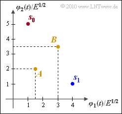
| − | + | We consider a binary message system $(M = 2)$ that is defined by the drawn 2D signal space constellation $(N = 2)$. The following applies to the two possible transmitted vectors that are directly coupled to the messages $m_0$ and $m_1$: | |
:$$\boldsymbol{ s }_0 \hspace{-0.1cm} \ =\ \hspace{-0.1cm} \sqrt {E} \cdot (1,\hspace{0.1cm} 5) \hspace{0.2cm} \Leftrightarrow \hspace{0.2cm} m_0 \hspace{0.05cm},$$ | :$$\boldsymbol{ s }_0 \hspace{-0.1cm} \ =\ \hspace{-0.1cm} \sqrt {E} \cdot (1,\hspace{0.1cm} 5) \hspace{0.2cm} \Leftrightarrow \hspace{0.2cm} m_0 \hspace{0.05cm},$$ | ||
:$$ \boldsymbol{ s }_1 \hspace{-0.1cm} \ =\ \hspace{-0.1cm} \sqrt {E} \cdot (4, \hspace{0.1cm}1) \hspace{0.2cm} \Leftrightarrow \hspace{0.2cm} m_1 \hspace{0.05cm}.$$ | :$$ \boldsymbol{ s }_1 \hspace{-0.1cm} \ =\ \hspace{-0.1cm} \sqrt {E} \cdot (4, \hspace{0.1cm}1) \hspace{0.2cm} \Leftrightarrow \hspace{0.2cm} m_1 \hspace{0.05cm}.$$ | ||
| − | + | The optimal decision boundary between the regions $I_0 ⇔ m_0$ and $I_1 ⇔ m_1$ is sought, whereby the following assumptions are made: | |
| − | * | + | * The following applies to subtasks '''(1)''' to '''(3)''' |
:$${\rm Pr}(m_0 ) = {\rm Pr}(m_1 ) = 0.5 | :$${\rm Pr}(m_0 ) = {\rm Pr}(m_1 ) = 0.5 | ||
\hspace{0.05cm}. $$ | \hspace{0.05cm}. $$ | ||
| − | * | + | * For subtasks '''(4)''' and '''(5)''', on the other hand, the following should apply: |
:$${\rm Pr}(m_0 ) = 0.817 \hspace{0.05cm},\hspace{0.2cm} {\rm Pr}(m_1 ) = 0.183\hspace{0.3cm} | :$${\rm Pr}(m_0 ) = 0.817 \hspace{0.05cm},\hspace{0.2cm} {\rm Pr}(m_1 ) = 0.183\hspace{0.3cm} | ||
\Rightarrow \hspace{0.3cm} {\rm ln} \hspace{0.15cm} \frac{{\rm Pr}( m_0)}{{\rm Pr}( m_1)} = | \Rightarrow \hspace{0.3cm} {\rm ln} \hspace{0.15cm} \frac{{\rm Pr}( m_0)}{{\rm Pr}( m_1)} = | ||
| Line 17: | Line 17: | ||
\hspace{0.05cm}.$$ | \hspace{0.05cm}.$$ | ||
| − | + | For AWGN noise with variance $\sigma_n^2$, the decision limit is the solution of the following vectorial equation with respect to the vector $(\rho_1, \rho_2)$: | |
:$$|| \boldsymbol{ s }_1||^2 - || \boldsymbol{ s }_0||^2 + 2 \cdot \sigma_n^2 \cdot {\rm ln} \hspace{0.15cm} \frac{{\rm Pr}( m_0)}{{\rm Pr}( m_1)} = | :$$|| \boldsymbol{ s }_1||^2 - || \boldsymbol{ s }_0||^2 + 2 \cdot \sigma_n^2 \cdot {\rm ln} \hspace{0.15cm} \frac{{\rm Pr}( m_0)}{{\rm Pr}( m_1)} = | ||
2 \cdot \boldsymbol{ \rho }^{\rm T} \cdot (\boldsymbol{ s }_1 - \boldsymbol{ s }_0)\hspace{0.05cm},\hspace{0.2cm} | 2 \cdot \boldsymbol{ \rho }^{\rm T} \cdot (\boldsymbol{ s }_1 - \boldsymbol{ s }_0)\hspace{0.05cm},\hspace{0.2cm} | ||
\boldsymbol{ \rho } = (\rho_1 , \hspace{0.1cm}\rho_2 )\hspace{0.05cm}.$$ | \boldsymbol{ \rho } = (\rho_1 , \hspace{0.1cm}\rho_2 )\hspace{0.05cm}.$$ | ||
| − | + | In addition, two received values | |
:$$\boldsymbol{ A }= \sqrt {E} \cdot (1.5, \hspace{0.1cm}2)\hspace{0.05cm}, \hspace{0.2cm} \boldsymbol{ B }= \sqrt {E} \cdot (3, \hspace{0.1cm}3.5) $$ | :$$\boldsymbol{ A }= \sqrt {E} \cdot (1.5, \hspace{0.1cm}2)\hspace{0.05cm}, \hspace{0.2cm} \boldsymbol{ B }= \sqrt {E} \cdot (3, \hspace{0.1cm}3.5) $$ | ||
| − | + | are drawn in the graphic. It must be checked whether these should be assigned to the regions $I_0$ $($and thus the message $m_0)$ or $I_1$ $($message $m_1)$ given the corresponding boundary conditions. | |
| Line 31: | Line 31: | ||
| − | '' | + | ''Notes:'' |
| − | * | + | * The exercise belongs to the chapter [[Digital_Signal_Transmission/Approximation_of_the_Error_Probability| Approximation of the Error Probability]]. |
| − | * | + | * For numeric calculations, the energy $E = 1$ can be set for simplification. |
| − | === | + | ===Questions=== |
<quiz display=simple> | <quiz display=simple> | ||
| − | { | + | {Where lies the optimal decision limit for equally probable symbols? At |
|type="[]"} | |type="[]"} | ||
+ $\rho_2 = 3/4 \cdot \rho_1 + 9/8$, | + $\rho_2 = 3/4 \cdot \rho_1 + 9/8$, | ||
| Line 46: | Line 46: | ||
- $\rho_2 = 3$. | - $\rho_2 = 3$. | ||
| − | { | + | {To which decision area does the received value $A = (1.5, \ \, 2)$ belong? |
|type="()"} | |type="()"} | ||
| − | - | + | - To decision area $I_0$, |
| − | + | + | + to decision area $I_1$. |
| − | { | + | {To which decision area does the received value $B = (3, \ \, 3.5)$ belong? |
|type="()"} | |type="()"} | ||
| − | + | + | + To decision area $I_0$, |
| − | - | + | - to decision area $I_1$. |
| − | { | + | {What is the equation of the decision line for ${\rm Pr}(m_0) = 0.817, \sigma_n = 1$? |
|type="()"} | |type="()"} | ||
- $\rho_2 = 3/4 \cdot \rho_1 + 9/8$, | - $\rho_2 = 3/4 \cdot \rho_1 + 9/8$, | ||
| Line 63: | Line 63: | ||
- $\rho_2 = 3/4 \cdot \rho_1$. | - $\rho_2 = 3/4 \cdot \rho_1$. | ||
| − | { | + | {Which decisions are made with these new regions $I_0$ and $I_1$? |
|type="[]"} | |type="[]"} | ||
| − | + | + | + The received vector $A$ is interpreted as message $m_0$. |
| − | - | + | - The received vector $A$ is interpreted as message $m_1$. |
| − | + | + | + The received vector $B$ is interpreted as message $m_0$. |
| − | - | + | - The received vector $B$ is interpreted as message $m_1$. |
</quiz> | </quiz> | ||
| − | === | + | ===Solution=== |
{{ML-Kopf}} | {{ML-Kopf}} | ||
| − | '''(1)''' | + | '''(1)''' With ${\rm Pr}(m_0) = {\rm Pr}(m_1) = 0.5$, the equation of the boundary line between the decision areas $I_0$ and $I_1$ reads: |
:$$|| \boldsymbol{ s }_1||^2 - || \boldsymbol{ s }_0||^2 = | :$$|| \boldsymbol{ s }_1||^2 - || \boldsymbol{ s }_0||^2 = | ||
2 \cdot \boldsymbol{ \rho }^{\rm T} \cdot (\boldsymbol{ s }_1 - \boldsymbol{ s }_0)\hspace{0.05cm}.$$ | 2 \cdot \boldsymbol{ \rho }^{\rm T} \cdot (\boldsymbol{ s }_1 - \boldsymbol{ s }_0)\hspace{0.05cm}.$$ | ||
| − | + | With the given vector values, i.e. the numerical values | |
:$$|| \boldsymbol{ s }_1||^2 = 4^2 + 1^2 = 17\hspace{0.05cm}, \hspace{0.2cm} | :$$|| \boldsymbol{ s }_1||^2 = 4^2 + 1^2 = 17\hspace{0.05cm}, \hspace{0.2cm} | ||
|| \boldsymbol{ s }_0||^2 = 1^2 + 5^2 = 26\hspace{0.05cm}, \hspace{0.2cm} | || \boldsymbol{ s }_0||^2 = 1^2 + 5^2 = 26\hspace{0.05cm}, \hspace{0.2cm} | ||
\boldsymbol{ s }_1 - \boldsymbol{ s }_0 = (3,\hspace{0.1cm}-4) \hspace{0.05cm}$$ | \boldsymbol{ s }_1 - \boldsymbol{ s }_0 = (3,\hspace{0.1cm}-4) \hspace{0.05cm}$$ | ||
| − | + | one obtains the following equation for the decision limits: | |
:$$3 \cdot \rho_1 - 4 \cdot \rho_2 = ({17-26})/{2} = - {9}/{2} | :$$3 \cdot \rho_1 - 4 \cdot \rho_2 = ({17-26})/{2} = - {9}/{2} | ||
\hspace{0.3cm}\Rightarrow \hspace{0.3cm}\rho_2 = 3/4 \cdot \rho_1 + 9/8 | \hspace{0.3cm}\Rightarrow \hspace{0.3cm}\rho_2 = 3/4 \cdot \rho_1 + 9/8 | ||
\hspace{0.05cm}.$$ | \hspace{0.05cm}.$$ | ||
| − | [[File:P_ID2033__Dig_A_4_6a.png|right|frame| | + | [[File:P_ID2033__Dig_A_4_6a.png|right|frame|Decision line and decision regions for $K=0$]] |
| − | + | The decision limit lies in the middle between $s_0$ and $s_1$ and is rotated by $90^\circ$ compared to the connecting line between the two symbols. It goes through the point $(2.5, \ \, 3)$. So the <u>first solution</u> is correct. | |
| − | + | Solution 2, on the other hand, describes the connecting line itself and $\rho_2 = 3$ is a horizontal line. | |
| − | '''(2)''' | + | '''(2)''' The decision area $I_1$ should of course contain the point $s_1$ ⇒ area below the decision line. Point $A = (1.5, \ \, 2)$ belongs to this decision domain, as shown in the graphic. This can be shown mathematically, since the decision line goes through the point $(1.5, \ \, 2.25)$, for example, and thus $(1.5, \ \, 2)$ lies below the decision line. So <u>solution 2</u> is correct. |
| − | '''(3)''' | + | '''(3)''' The decision line also goes through the point $(3, \ \, 3.375)$. $B = (3, \ \, 3.5)$ lies above and therefore belongs to the decision region $I_0$ according to <u>solution 1</u>. |
| − | '''(4)''' | + | '''(4)''' According to the equation in the information section and the calculations for subtask (1), the following now applies: |
| − | [[File:P_ID2034__Dig_A_4_6c.png|right|frame| | + | [[File:P_ID2034__Dig_A_4_6c.png|right|frame|Decision areas for different $K$ values]] |
:$$|| \boldsymbol{ s }_1||^2 - || \boldsymbol{ s }_0||^2 + 2 \cdot \sigma_n^2 \cdot {\rm ln} \hspace{0.15cm} \frac{{\rm Pr}( m_0)}{{\rm Pr}( m_1)} = | :$$|| \boldsymbol{ s }_1||^2 - || \boldsymbol{ s }_0||^2 + 2 \cdot \sigma_n^2 \cdot {\rm ln} \hspace{0.15cm} \frac{{\rm Pr}( m_0)}{{\rm Pr}( m_1)} = | ||
2 \cdot \boldsymbol{ \rho }^{\rm T} \cdot (\boldsymbol{ s }_1 - \boldsymbol{ s }_0)\hspace{0.05cm}.$$ | 2 \cdot \boldsymbol{ \rho }^{\rm T} \cdot (\boldsymbol{ s }_1 - \boldsymbol{ s }_0)\hspace{0.05cm}.$$ | ||
| − | + | With $|| \boldsymbol{ s }_1||^2 = 17$, $|| \boldsymbol{ s }_0||^2 = 26$, $ \boldsymbol{ s }_1 \, –\boldsymbol{ s }_0 = (3, \ \, –4)$ we obtain: | |
:$$\rho_2 = 3/4 \cdot \rho_1 + 9/8 - K /8 | :$$\rho_2 = 3/4 \cdot \rho_1 + 9/8 - K /8 | ||
\hspace{0.05cm}.$$ | \hspace{0.05cm}.$$ | ||
| − | + | The following abbreviation was used here: | |
:$$K = 2 \cdot \sigma_n^2 \cdot {\rm ln} \hspace{0.15cm} \frac{{\rm Pr}( m_0)}{{\rm Pr}( m_1)} = | :$$K = 2 \cdot \sigma_n^2 \cdot {\rm ln} \hspace{0.15cm} \frac{{\rm Pr}( m_0)}{{\rm Pr}( m_1)} = | ||
2 \cdot 1^2 \cdot 1.5 = 3 \hspace{0.05cm}.$$ | 2 \cdot 1^2 \cdot 1.5 = 3 \hspace{0.05cm}.$$ | ||
| − | + | From this it follows: | |
:$$\rho_2 = 3/4 \cdot \rho_1 + 9/8 - 3 /8 = 3/4 \cdot \rho_1 + 3/4 | :$$\rho_2 = 3/4 \cdot \rho_1 + 9/8 - 3 /8 = 3/4 \cdot \rho_1 + 3/4 | ||
\hspace{0.05cm}.$$ | \hspace{0.05cm}.$$ | ||
| − | + | The decision line is shifted down by $3/8$ (black curve, labeled "$K = 3$" in the graphic). So <u>solution 2</u> is correct. | |
| − | * | + | *The first equation describes the optimal decision boundary for equally probable symbols ($K = 0$, dashed gray). |
| − | * | + | *The third equation is valid for $K = \, –3$. This results with $\sigma_n^2 = 1$ for the symbol probabilities ${\rm Pr}(m_1) \approx 0.817$ and ${\rm Pr}(m_0) \approx 0.138$ (green curve). |
| − | * | + | *The violet straight line results with $K = 9$, i.e. with the same probabilities as for the black curve, but now with the variance $\sigma_n^2 = 3$. |
| − | '''(5)''' | + | '''(5)''' The graphic above already shows that both $A$ and $B$ now belong to the decision regio $I_0$. <u>Solutions 1 and 3</u> are correct. |
{{ML-Fuß}} | {{ML-Fuß}} | ||
Revision as of 14:54, 5 July 2022
We consider a binary message system $(M = 2)$ that is defined by the drawn 2D signal space constellation $(N = 2)$. The following applies to the two possible transmitted vectors that are directly coupled to the messages $m_0$ and $m_1$:
- $$\boldsymbol{ s }_0 \hspace{-0.1cm} \ =\ \hspace{-0.1cm} \sqrt {E} \cdot (1,\hspace{0.1cm} 5) \hspace{0.2cm} \Leftrightarrow \hspace{0.2cm} m_0 \hspace{0.05cm},$$
- $$ \boldsymbol{ s }_1 \hspace{-0.1cm} \ =\ \hspace{-0.1cm} \sqrt {E} \cdot (4, \hspace{0.1cm}1) \hspace{0.2cm} \Leftrightarrow \hspace{0.2cm} m_1 \hspace{0.05cm}.$$
The optimal decision boundary between the regions $I_0 ⇔ m_0$ and $I_1 ⇔ m_1$ is sought, whereby the following assumptions are made:
- The following applies to subtasks (1) to (3)
- $${\rm Pr}(m_0 ) = {\rm Pr}(m_1 ) = 0.5 \hspace{0.05cm}. $$
- For subtasks (4) and (5), on the other hand, the following should apply:
- $${\rm Pr}(m_0 ) = 0.817 \hspace{0.05cm},\hspace{0.2cm} {\rm Pr}(m_1 ) = 0.183\hspace{0.3cm} \Rightarrow \hspace{0.3cm} {\rm ln} \hspace{0.15cm} \frac{{\rm Pr}( m_0)}{{\rm Pr}( m_1)} = 1.5 \hspace{0.05cm}.$$
For AWGN noise with variance $\sigma_n^2$, the decision limit is the solution of the following vectorial equation with respect to the vector $(\rho_1, \rho_2)$:
- $$|| \boldsymbol{ s }_1||^2 - || \boldsymbol{ s }_0||^2 + 2 \cdot \sigma_n^2 \cdot {\rm ln} \hspace{0.15cm} \frac{{\rm Pr}( m_0)}{{\rm Pr}( m_1)} = 2 \cdot \boldsymbol{ \rho }^{\rm T} \cdot (\boldsymbol{ s }_1 - \boldsymbol{ s }_0)\hspace{0.05cm},\hspace{0.2cm} \boldsymbol{ \rho } = (\rho_1 , \hspace{0.1cm}\rho_2 )\hspace{0.05cm}.$$
In addition, two received values
- $$\boldsymbol{ A }= \sqrt {E} \cdot (1.5, \hspace{0.1cm}2)\hspace{0.05cm}, \hspace{0.2cm} \boldsymbol{ B }= \sqrt {E} \cdot (3, \hspace{0.1cm}3.5) $$
are drawn in the graphic. It must be checked whether these should be assigned to the regions $I_0$ $($and thus the message $m_0)$ or $I_1$ $($message $m_1)$ given the corresponding boundary conditions.
Notes:
- The exercise belongs to the chapter Approximation of the Error Probability.
- For numeric calculations, the energy $E = 1$ can be set for simplification.
Questions
Solution
- $$|| \boldsymbol{ s }_1||^2 - || \boldsymbol{ s }_0||^2 = 2 \cdot \boldsymbol{ \rho }^{\rm T} \cdot (\boldsymbol{ s }_1 - \boldsymbol{ s }_0)\hspace{0.05cm}.$$
With the given vector values, i.e. the numerical values
- $$|| \boldsymbol{ s }_1||^2 = 4^2 + 1^2 = 17\hspace{0.05cm}, \hspace{0.2cm} || \boldsymbol{ s }_0||^2 = 1^2 + 5^2 = 26\hspace{0.05cm}, \hspace{0.2cm} \boldsymbol{ s }_1 - \boldsymbol{ s }_0 = (3,\hspace{0.1cm}-4) \hspace{0.05cm}$$
one obtains the following equation for the decision limits:
- $$3 \cdot \rho_1 - 4 \cdot \rho_2 = ({17-26})/{2} = - {9}/{2} \hspace{0.3cm}\Rightarrow \hspace{0.3cm}\rho_2 = 3/4 \cdot \rho_1 + 9/8 \hspace{0.05cm}.$$
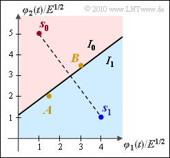
The decision limit lies in the middle between $s_0$ and $s_1$ and is rotated by $90^\circ$ compared to the connecting line between the two symbols. It goes through the point $(2.5, \ \, 3)$. So the first solution is correct.
Solution 2, on the other hand, describes the connecting line itself and $\rho_2 = 3$ is a horizontal line.
(2) The decision area $I_1$ should of course contain the point $s_1$ ⇒ area below the decision line. Point $A = (1.5, \ \, 2)$ belongs to this decision domain, as shown in the graphic. This can be shown mathematically, since the decision line goes through the point $(1.5, \ \, 2.25)$, for example, and thus $(1.5, \ \, 2)$ lies below the decision line. So solution 2 is correct.
(3) The decision line also goes through the point $(3, \ \, 3.375)$. $B = (3, \ \, 3.5)$ lies above and therefore belongs to the decision region $I_0$ according to solution 1.
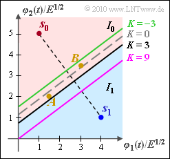
(4) According to the equation in the information section and the calculations for subtask (1), the following now applies:
- $$|| \boldsymbol{ s }_1||^2 - || \boldsymbol{ s }_0||^2 + 2 \cdot \sigma_n^2 \cdot {\rm ln} \hspace{0.15cm} \frac{{\rm Pr}( m_0)}{{\rm Pr}( m_1)} = 2 \cdot \boldsymbol{ \rho }^{\rm T} \cdot (\boldsymbol{ s }_1 - \boldsymbol{ s }_0)\hspace{0.05cm}.$$
With $|| \boldsymbol{ s }_1||^2 = 17$, $|| \boldsymbol{ s }_0||^2 = 26$, $ \boldsymbol{ s }_1 \, –\boldsymbol{ s }_0 = (3, \ \, –4)$ we obtain:
- $$\rho_2 = 3/4 \cdot \rho_1 + 9/8 - K /8 \hspace{0.05cm}.$$
The following abbreviation was used here:
- $$K = 2 \cdot \sigma_n^2 \cdot {\rm ln} \hspace{0.15cm} \frac{{\rm Pr}( m_0)}{{\rm Pr}( m_1)} = 2 \cdot 1^2 \cdot 1.5 = 3 \hspace{0.05cm}.$$
From this it follows:
- $$\rho_2 = 3/4 \cdot \rho_1 + 9/8 - 3 /8 = 3/4 \cdot \rho_1 + 3/4 \hspace{0.05cm}.$$
The decision line is shifted down by $3/8$ (black curve, labeled "$K = 3$" in the graphic). So solution 2 is correct.
- The first equation describes the optimal decision boundary for equally probable symbols ($K = 0$, dashed gray).
- The third equation is valid for $K = \, –3$. This results with $\sigma_n^2 = 1$ for the symbol probabilities ${\rm Pr}(m_1) \approx 0.817$ and ${\rm Pr}(m_0) \approx 0.138$ (green curve).
- The violet straight line results with $K = 9$, i.e. with the same probabilities as for the black curve, but now with the variance $\sigma_n^2 = 3$.
(5) The graphic above already shows that both $A$ and $B$ now belong to the decision regio $I_0$. Solutions 1 and 3 are correct.


