Difference between revisions of "Channel Coding/Decoding of Linear Block Codes"
| Line 96: | Line 96: | ||
::<math>\underline{s} = (0, 0, 0) \hspace{0.10cm} \Rightarrow\hspace{0.10cm}{\rm no\hspace{0.15cm} correction}\hspace{0.05cm};\hspace{0.8cm}\underline{s} = (1, 0, 0)\hspace{0.10cm} \Rightarrow\hspace{0.10cm}{\rm invert}\hspace{0.15cm}p_1\hspace{0.05cm};</math> | ::<math>\underline{s} = (0, 0, 0) \hspace{0.10cm} \Rightarrow\hspace{0.10cm}{\rm no\hspace{0.15cm} correction}\hspace{0.05cm};\hspace{0.8cm}\underline{s} = (1, 0, 0)\hspace{0.10cm} \Rightarrow\hspace{0.10cm}{\rm invert}\hspace{0.15cm}p_1\hspace{0.05cm};</math> | ||
| − | ::<math>\underline{s} =(0, 0, 1)\hspace{0.10cm} \Rightarrow\hspace{0.10cm} {\rm invert}\hspace{0.15cm}p_3\hspace{0.05cm};\hspace{1. | + | ::<math>\underline{s} =(0, 0, 1)\hspace{0.10cm} \Rightarrow\hspace{0.10cm} {\rm invert}\hspace{0.15cm}p_3\hspace{0.05cm};\hspace{1.63cm}\underline{s} = (1, 0, 1)\hspace{0.10cm} \Rightarrow\hspace{0.10cm} {\rm invert}\hspace{0.15cm}u_1\hspace{0.05cm};</math> |
| − | ::<math>\underline{s} =(0, 1, 0)\hspace{0.10cm} \Rightarrow\hspace{0.10cm} {\rm invert}\hspace{0.15cm}p_2\hspace{0.05cm};\hspace{1. | + | ::<math>\underline{s} =(0, 1, 0)\hspace{0.10cm} \Rightarrow\hspace{0.10cm} {\rm invert}\hspace{0.15cm}p_2\hspace{0.05cm};\hspace{1.63cm}\underline{s} = (1, 1, 0)\hspace{0.10cm} \Rightarrow\hspace{0.10cm} {\rm invert}\hspace{0.15cm}u_3\hspace{0.05cm};</math> |
| − | ::<math>\underline{s} =(0, 1, 1)\hspace{0.10cm} \Rightarrow\hspace{0.10cm} {\rm invert}\hspace{0.15cm}u_4\hspace{0.05cm};\hspace{1. | + | ::<math>\underline{s} =(0, 1, 1)\hspace{0.10cm} \Rightarrow\hspace{0.10cm} {\rm invert}\hspace{0.15cm}u_4\hspace{0.05cm};\hspace{1.63cm}\underline{s} = (1, 1, 1)\hspace{0.10cm} \Rightarrow\hspace{0.10cm} {\rm invert}\hspace{0.15cm}u_2\hspace{0.05cm}. </math>}}<br> |
== Generalization of syndrome coding == | == Generalization of syndrome coding == | ||
Revision as of 14:49, 12 July 2022
Contents
Block diagram and requirements
We start from the block diagram already shown in the chapter "Channel Models and Decision Structures" where the digital channel model used is mostly the "Binary Symmetric Channel" $\rm (BSC)$.
For code word estimation, we use the "Maximum Likelihood Decision" $\rm (ML)$, which for binary codes ⇒ $\underline{x} \in {\rm GF}(2^n)$ at the block level gives the same result as the "MAP Receiver".
The task of the channel decoder can be described as follows:
- The vector $\underline{v}$ after decoding (at the sink) should match the information word $\underline{u}$ as well as possible.
- That is: The block error probability should be as small as possible:
- \[{ \rm Pr(block\:error)} = { \rm Pr}( \underline{v} \ne \underline{u}) \stackrel{!}{=} { \rm minimum}\hspace{0.05cm}.\]
- Because of assignments $\underline{x} = {\rm enc}(\underline{u})$ resp. $\underline{v} = {\rm enc}^{-1}(\underline{z})$ also holds:
- \[{ \rm Pr(block\:error)} = { \rm Pr}( \underline{z} \ne \underline{x}) \stackrel{!}{=} { \rm minimum}\hspace{0.05cm}.\]
- Sought is the most likely sent code word $\underline{y} = \underline{x} +\underline{e}$ for the given received word $\underline{x}_i$, which is passed on as result $\underline{z}$:
- \[\underline{z} = {\rm arg} \max_{\underline{x}_{\hspace{0.03cm}i} \hspace{0.05cm} \in \hspace{0.05cm} \mathcal{C}} \hspace{0.1cm} {\rm Pr}( \underline{x}_{\hspace{0.03cm}i} \hspace{0.05cm}|\hspace{0.05cm} \underline{y} ) \hspace{0.05cm}.\]
- For the BSC model, both $\underline{x}_i \in {\rm GF}(2^n)$ and $\underline{y} \in {\rm GF}(2^n)$, so the maximum likelihood decision rule can also be written using the "Hamming distance" $d_{\rm H}( \underline{y}, \, \underline{x}_i)$:
- \[\underline{z} = {\rm arg} \min_{\underline{x}_{\hspace{0.03cm}i} \hspace{0.05cm} \in \hspace{0.05cm} \mathcal{C}} \hspace{0.1cm} d_{\rm H}(\underline{y} \hspace{0.05cm}, \hspace{0.1cm}\underline{x}_{\hspace{0.03cm}i})\hspace{0.05cm}.\]
Principle of syndrome decoding
Assumed here is a $(n, \, k)$ block code with the parity-check matrix $\boldsymbol{\rm H}$ and the systematic code words
- \[\underline{x}\hspace{0.05cm} = (x_1, x_2, \hspace{0.05cm}\text{...} \hspace{0.05cm}, x_i, \hspace{0.05cm}\text{...} \hspace{0.05cm}, x_n) = (u_1, u_2, \hspace{0.05cm}\text{...} \hspace{0.05cm}, u_k, p_1, \hspace{0.05cm}\text{...} \hspace{0.05cm}, p_{n-k})\hspace{0.05cm}. \]
With the error vector $\underline{e}$ then applies to the received word:
- \[\underline{y} = \underline{x} + \underline{e} \hspace{0.05cm}, \hspace{0.4cm} \underline{y} \in \hspace{0.1cm} {\rm GF}(2^n) \hspace{0.05cm}, \hspace{0.4cm} \underline{x} \in \hspace{0.1cm} {\rm GF}(2^n) \hspace{0.05cm}, \hspace{0.4cm} \underline{e} \in \hspace{0.1cm} {\rm GF}(2^n) \hspace{0.05cm}.\]
A bit error at position $i$ ⇒ $y_i ≠ x_i$ is expressed by the error coefficient $e_i = 1$.
$\text{Definition:}$ The syndrome $\underline{s} = (s_0, s_1, \hspace{0.05cm}\text{...} \hspace{0.05cm}, s_{m-1})$ is calculated (as row resp. column vector) from the received word $\underline{y}$ and the parity-check matrix $\boldsymbol{\rm H}$ as follows:
- \[\underline{s} = \underline{y} \cdot { \boldsymbol{\rm H} }^{\rm T}\hspace{0.3cm}{\rm bzw.}\hspace{0.3cm} \underline{s}^{\rm T} = { \boldsymbol{\rm H} } \cdot \underline{y}^{\rm T}\hspace{0.05cm}.\]
- The vector length of $\underline{s}$ is equal to $m = n-k$ $($row number of $\boldsymbol{\rm H})$.
The syndrome $\underline{s}$ shows the following characteristics:
- Because of the equation $\underline{x} \cdot { \boldsymbol{\rm H}}^{\rm T} = \underline{0}$ the syndrome $\underline{s}$ does not depend on the code word $\underline{x}$ but solely on the error vector $\underline{e}$:
- \[\underline{s} = \underline{y} \cdot { \boldsymbol{\rm H}}^{\rm T} = \hspace{0.05cm} \underline{x} \cdot { \boldsymbol{\rm H}}^{\rm T} + \hspace{0.05cm} \underline{e} \cdot { \boldsymbol{\rm H}}^{\rm T} = \hspace{0.05cm} \underline{e} \cdot { \boldsymbol{\rm H}}^{\rm T} \hspace{0.05cm}.\]
- For sufficiently few bit errors, $\underline{s}$ provides a clear indication of the error locations, allowing full error correction.
$\text{Example 1:}$ Starting from the systematic $\text{(7, 4, 3)}$ Hamming code, the following result is obtained for the received vector $\underline{y} = (0, 1, 1, 1, 0, 0, 1)$:
- \[{ \boldsymbol{\rm H} } \cdot \underline{y}^{\rm T} = \begin{pmatrix} 1 &1 &1 &0 &1 &0 &0\\ 0 &1 &1 &1 &0 &1 &0\\ 1 &1 &0 &1 &0 &0 &1 \end{pmatrix} \cdot \begin{pmatrix} 0 \\ 1 \\ 1 \\ 1 \\ 0 \\ 0 \\ 1 \end{pmatrix} = \begin{pmatrix} 0 \\ 1 \\ 1 \end{pmatrix} = \underline{s}^{\rm T} \hspace{0.05cm}.\]
Comparing the syndrome with the parity-check equations of the Hamming code, we see that
- most likely the fourth symbol $(x_4 = u_4)$ of the code word has been corrupted,
- the code word estimator will thus yield the result $\underline{z} = (0, 1, 1, 0, 0, 0, 1)$,
- the decision is correct only if only one bit was corrupted during transmission.
Below are the required corrections for the $\text{(7, 4, 3)}$ Hamming code resulting from the calculated syndrome $\underline{s}$ corresponding to the columns of the parity-check matrix:
- \[\underline{s} = (0, 0, 0) \hspace{0.10cm} \Rightarrow\hspace{0.10cm}{\rm no\hspace{0.15cm} correction}\hspace{0.05cm};\hspace{0.8cm}\underline{s} = (1, 0, 0)\hspace{0.10cm} \Rightarrow\hspace{0.10cm}{\rm invert}\hspace{0.15cm}p_1\hspace{0.05cm};\]
- \[\underline{s} =(0, 0, 1)\hspace{0.10cm} \Rightarrow\hspace{0.10cm} {\rm invert}\hspace{0.15cm}p_3\hspace{0.05cm};\hspace{1.63cm}\underline{s} = (1, 0, 1)\hspace{0.10cm} \Rightarrow\hspace{0.10cm} {\rm invert}\hspace{0.15cm}u_1\hspace{0.05cm};\]
- \[\underline{s} =(0, 1, 0)\hspace{0.10cm} \Rightarrow\hspace{0.10cm} {\rm invert}\hspace{0.15cm}p_2\hspace{0.05cm};\hspace{1.63cm}\underline{s} = (1, 1, 0)\hspace{0.10cm} \Rightarrow\hspace{0.10cm} {\rm invert}\hspace{0.15cm}u_3\hspace{0.05cm};\]
- \[\underline{s} =(0, 1, 1)\hspace{0.10cm} \Rightarrow\hspace{0.10cm} {\rm invert}\hspace{0.15cm}u_4\hspace{0.05cm};\hspace{1.63cm}\underline{s} = (1, 1, 1)\hspace{0.10cm} \Rightarrow\hspace{0.10cm} {\rm invert}\hspace{0.15cm}u_2\hspace{0.05cm}. \]
Generalization of syndrome coding
We continue to assume the BSC channel model. This means:
- The receive vector $\underline{y}$ and the error vector $\underline{e}$ are elements of ${\rm GF}(2^n)$.
- The possible codewords $\underline{x}_i$ belong to the code $\mathcal{C}$, which spans a $(n-k)$ dimensional subspace of ${\rm GF}(2^n)$ .
Under this assumption, we briefly summarize again the results of the last pages:
- Syndrome decoding is a realization possibility of maximum likelihood detection of block codes. One decides on the codeword $\underline{x}_i$ with the least Hamming distance to the receiving word $\underline{y}$ :
- \[\underline{z} = {\rm arg} \min_{\underline{x}_{\hspace{0.03cm}i} \hspace{0.05cm} \in \hspace{0.05cm} \mathcal{C}} \hspace{0.1cm} d_{\rm H}(\underline{y} \hspace{0.05cm}, \hspace{0.1cm}\underline{x}_{\hspace{0.03cm}i})\hspace{0.05cm}.\]
- But the syndrome decoding is also the search for the most probable error vector $\underline{e}$ that satisfies the condition $\underline{e} \cdot { \boldsymbol{\rm H}}^{\rm T} = \underline{s}$ . The syndrome is thereby determined by the equation $\underline{s} = \underline{y} \cdot { \boldsymbol{\rm H}}^{\rm T} $ .
- With the Hamming weight $w_{\rm H}(\underline{e})$ the second interpretation can also be mathematically formulated as follows:
- \[\underline{z} = \underline{y} + {\rm arg} \min_{\underline{e}_{\hspace{0.03cm}i} \hspace{0.05cm} \in \hspace{0.05cm} {\rm GF}(2^n)} \hspace{0.1cm} w_{\rm H}(\underline{e}_{\hspace{0.03cm}i})\hspace{0.05cm}.\]
$\text{Conclusion:}$ Note that the error vector $\underline{e}$ as well as the receive vector $\underline{y}$ is an element of ${\rm GF}(2^n)$ unlike the syndrome $\underline{s} \in {\rm GF}(2^m)$ with number $m = n-k$ of parity-check equations. This means,
- that the association between the syndrome $\underline{s}$ and the error vector $\underline{e}$ is not unique, but
- that each $2^k$ error vectors lead to the same syndrome $\underline{s}$ which one groups together into a coset
.
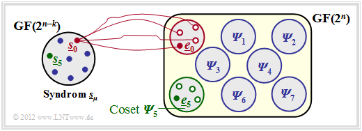
$\text{Example 2:}$ The facts shall be illustrated here by the example $n = 5, \ k = 2$ ⇒ $m = n-k = 3$ .
You can see from this graph:
- The $2^n = 32$ possible error vectors $\underline{e}$ are divided into $2^m = 8$ cosets ${\it \Psi}_0$, ... , ${\it \Psi}_7$ split.
- Explicitly drawn here are only the cosets ${\it \Psi}_0$ and ${\it \Psi}_5$.
- All $2^k = 4$ error vectors of the coset ${\it \Psi}_\mu$ lead to the syndrome $\underline{s}_\mu$.
- Each minor class ${\it \Psi}_\mu$ has a leader $\underline{e}_\mu$, namely the one with the minimum Hamming weight.
$\text{Example 3:}$ Starting from the systematic $\text{(5, 2, 3)}$ code $\mathcal{C} = \big \{ (0, 0, 0, 0, 0) \hspace{0.05cm},\hspace{0.15cm}(0, 1, 0, 1, 1) \hspace{0.05cm},\hspace{0.15cm}(1, 0, 1, 1, 0) \hspace{0.05cm},\hspace{0.15cm}(1, 1, 1, 0, 1) \big \}$ the syndrome decoding procedure is now described in detail.
The generator matrix and the parity-check matrix are:
- \[{ \boldsymbol{\rm G} } = \begin{pmatrix} 1 &0 &1 &1 &0 \\ 0 &1 &0 &1 &1 \end{pmatrix} \hspace{0.05cm},\]
- \[{ \boldsymbol{\rm H} } = \begin{pmatrix} 1 &0 &1 &0 &0 \\ 1 &1 &0 &1 &0 \\ 0 &1 &0 &0 &1 \end{pmatrix} \hspace{0.05cm}.\]
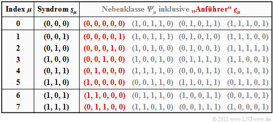
The table summarizes the final result. Note:
- The index $\mu$ is not identical to the binary value of $\underline{s}_\mu$.
- The order is rather given by the number of ones in the minor class leader $\underline{e}_\mu$.
- For example, the syndrome $\underline{s}_5 = (1, 1, 0)$ and the syndrome $\underline{s}_6 = (1, 0, 1)$.
To derive this table, note:
- The row 1 refers to the syndrome $\underline{s}_0 = (0, 0, 0)$ and the associated cosets ${\it \Psi}_0$. The most likely error sequence here is $(0, 0, 0, 0)$ ⇒ no bit error, which we call the coset leader $\underline{e}_0$ .
- The other entries in the first row, namely $(1, 0, 1, 1, 0 )$, $(0, 1, 0, 1, 1)$ and $(1, 1, 1, 0, 1 )$, each yield the syndrome $\underline{s}_0 = (0, 0, 0)$, but yield only with at least three bit errors and are correspondingly unlikely.
- In rows 2 to 6, the respective coset leader $\underline{e}_\mu$ contains exactly a single one $(\mu = 1$, ... , $5)$. Here $\underline{e}_\mu$ is always the most likely error pattern of the class ${\it \Psi}_\mu$. The other group members result only with at least two bit errors.
- The syndrome $\underline{s}_6 = (1, 0, 1)$ is not possible with only one bit error. In creating the table, we then considered all $5\text{ over }2 = 10$ error patterns $\underline{e}$ with weight $w_{\rm H}(\underline{e}) = 2$ .
- The first found sequence with syndrome $\underline{s}_6 = (1, 0, 1)$ was chosen as coset leader $\underline{e}_6 = (1, 1, 0, 0)$ . With a different probing order, the sequence $(0, 0, 1, 0, 1)$ could also have resulted from ${\it \Psi}_6$ .
- Similar procedure was followed in determining the leader $\underline{e}_7 = (0, 1, 1, 0, 0)$ of the cosets class ${\it \Psi}_7$ characterized by the uniform syndrome $\underline{s}_7 = (1, 1, 1)$ . Also in the class ${\it \Psi}_7$ there is another sequence with Hamming weight $w_{\rm H}(\underline{e}) = 2$, namely $(1, 0, 0, 0, 1)$.
The above table only needs to be created once and can be used as often as desired. First, the syndrome must be determined. This is for example for the receive vector $\underline{y} = (0, 1, 0, 0, 1)$:
- \[\underline{s} = \underline{y} \cdot { \boldsymbol{\rm H} }^{\rm T} = \begin{pmatrix} 0 &1 &0 &0 &1 \end{pmatrix} \cdot \begin{pmatrix} 1 &1 &0 \\ 0 &1 &1 \\ 1 &0 &0 \\ 0 &1 &0 \\ 0 &0 &1 \\ \end{pmatrix} = \begin{pmatrix} 0 &1 &0 \end{pmatrix}= \underline{s}_2 \hspace{0.05cm}.\]
Using the coset leader $\underline{e}_2 = (0, 0, 0, 1, 0)$ from the above table $($red entry for $\mu =2)$ finally arrives at the decoding result:
- \[\underline{z} = \underline{y} + \underline{e}_2 = (0,\hspace{0.05cm} 1,\hspace{0.05cm} 0,\hspace{0.05cm} 0,\hspace{0.05cm} 1) + (0,\hspace{0.05cm} 0,\hspace{0.05cm} 0,\hspace{0.05cm} 1,\hspace{0.05cm} 0) = (0,\hspace{0.05cm} 1,\hspace{0.05cm} 0,\hspace{0.05cm} 1,\hspace{0.05cm} 1) \hspace{0.05cm}.\]
$\text{Conclusion:}$ From these examples it is already clear that the syndrome decoding involves a considerable effort is connected, if one cannot use certain characteristics as with cyclic codes:
- For large block code lengths, this method fails completely. Thus, to decode a BCH codes – the abbreviation stands for their inventors Bose, Chaudhuri and Hocquenghem – with code parameters $n = 511$, $k = 259$ and $d_{\rm min} = 61$ exactly $2^{511-259} \approx 10^{76}$ evaluate and save error patterns of length $511$ .
- Happily, however, there are special decoding algorithms for these and also for other codes of large block length, which lead to success with less effort
.
Coding gain - bit error rate with AWGN
We now consider the Bit error rate for the following constellation:
- Hamming code $\text{HC (7, 4, 3)}$,
- AWGN–channel, characterized by the quotient $E_{\rm B}/N_0$ (in dB),
- Maximum Likelihood Detection (ML) with Hard Decision and Soft Decision respectively.
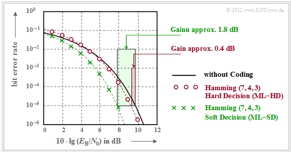
It should be noted with regard to this graph:
- The black comparison curve applies, for example, to binary phase modulation (BPSK) without coding. For this one needs for the bit error rate $10^{-5}$ about $10 \cdot \lg \, E_{\rm B}/N_0 = 9.6 \, \rm dB$.
- The red circles apply to the $\text{(7, 4, 3)}$ code and hard decisions of the maximum likelihood decoder $\text{(ML–HD)}$. Syndrome decoding is a possible realization form for this.
- This configuration brings only for $10 \cdot \lg \, E_{\rm B}/N_0 >6 \, \rm dB$ an improvement over the comparison system. For $\rm BER =10^{-5}$ one only needs $10 \cdot \lg \, E_{\rm B}/N_0 \approx 9.2 \, \rm dB$.
- The green crosses for the Hamming–Code and Soft–Decision $\text{(ML–SD)}$ are below the comparison curve throughout the range. For $\rm BER =10^{-5}$ this gives $10 \cdot \lg \, E_{\rm B}/N_0 \approx 7.8 \, \rm dB$.
$\text{Definition:}$ As coding gain of a system configuration (characterized by its code and the way it is decoded) we refer to the smaller $10 \cdot \lg \, E_{\rm B}/N_0$ required for a given bit error rate $\rm (BER)$ compared to the comparison system (without coding):
- \[G_{\rm Code} (\hspace{0.05cm}{\rm System}\hspace{0.05cm}\vert\hspace{0.05cm}{\rm BER}\hspace{0.05cm}) =10 \cdot {\rm lg}\hspace{0.1cm}{E}_{\rm B}/N_0 \hspace{0.15cm}(\hspace{0.05cm}{\rm without\hspace{0.1cm} coding}\hspace{0.05cm}\vert\hspace{0.05cm}{\rm BER}\hspace{0.05cm})- 10 \cdot {\rm lg}\hspace{0.1cm}{E}_{\rm B}/N_0 \hspace{0.15cm}(\hspace{0.05cm}{\rm System}\hspace{0.05cm}\vert\hspace{0.05cm}{\rm BER}\hspace{0.05cm}) \hspace{0.05cm}. \]
Applied to the above graph, one obtains:
\[G_{\rm Code} (\hspace{0.05cm}{\rm Hamming \hspace{0.1cm}(7,\hspace{0.02cm}4,\hspace{0.02cm}3), ML-HD}\hspace{0.05cm}|\hspace{0.05cm}{\rm BER} = 10^{-5}\hspace{0.05cm}) = 0.4\ {\rm dB}\hspace{0.05cm},\]
\[G_{\rm Code} (\hspace{0.05cm}{\rm Hamming \hspace{0.1cm}(7,\hspace{0.02cm}4,\hspace{0.02cm}3), ML-SD}\hspace{0.05cm}|\hspace{0.05cm}{\rm BER} = 10^{-5}\hspace{0.05cm}) = 1.8\ {\rm dB}\hspace{0.05cm}.\]
Decoding at the Binary Erasure Channel
Finally, it will be shown to what extent the decoder has to be modified if instead of thes "BSC–Modells" (TOTER LINK) (Binary Symmetric Channel ) the "BEC–Kanalmodell" (TOTER LINK) (Binary Erasure Channel ) is used, which does not produce errors but marks uncertain bits as erasures.
$\text{Example 4:}$ Without limiting generality, as in $\text{"Example 3"}$ we again consider the systematic $\text{(5, 2, 3)}$–block code
- $$\mathcal{C} = \big \{ (0, 0, 0, 0, 0) \hspace{0.05cm},\hspace{0.15cm}(0, 1, 0, 1, 1) \hspace{0.05cm},\hspace{0.15cm}(1, 0, 1, 1, 0) \hspace{0.05cm},\hspace{0.15cm}(1, 1, 1, 0, 1) \big \}.$$
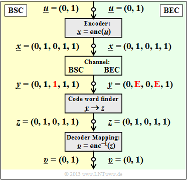
Die Grafik zeigt das Systemmodell und gibt beispielhafte Werte für die einzelnen Vektoren wider.
- The left part of the picture (yellow background) is valid for "BSC" with a bit error $0 → 1$ at the third bit.
- The right part of the picture (green background) is for "BEC" and shows two Erasures $\rm 1 → E$ at bit 2 and bit 4.
One recognizes:
- With BSC only one bit error can be corrected due to $d_{\rm min} = 3$ ($t = 1$, marked in red). If one restricts oneself to error detection, this works up to $e= d_{\rm min} -1 = 2$ bit errors.
- For BEC, error detection makes no sense, because already the channel locates an uncertain bit as an Erasure $\rm E$ . The zeros and ones in the BEC received word $\underline{y}$ are safe. Therefore the error correction works here up to $e = 2$ erasures with certainty.
- Also $e = 3$ erasures are sometimes still correctable. So $\underline{y} \rm = (E, E, E, 1, 1)$ to $\underline{z} \rm = (0, 1, 0, 1, 1)$ to be corrected since no second codeword ends with two ones $\underline{y} \rm = (0, E, 0, E, E)$ but is not correctable because of the all zero word allowed in the code.
- If it is ensured that there are no more than two erasures in any received word, the BEC block error probability ${\rm Pr}(\underline{z} \ne \underline{x}) = {\rm Pr}(\underline{v} \ne \underline{u}) \equiv 0$. In contrast, the corresponding block error probability in the BSC model always has a value greater than $0$.
Since after the BEC each received word is either decoded correctly or not at all, we call here the block $\underline{y} → \underline{z}$ in the future "codeword finder". An "estimation" takes place only in the BSC model.
But how does the decoding of a received word $\underline{y}$ with erasures work algorithmically?
$\text{Example 5:}$ Starting from the received word $\underline{y} \rm = (0, E, 0, E, 1)$ in $\text{example 4}$ we formally set the output of the codeword finder to $\underline{z} \rm = (0, z_2, 0, z_4, 1)$, where the symbols $z_2 \in \{0, \, 1\}$ and $z_4 \in \{0, \, 1\}$ are to be determined according to the following equation:
- \[\underline{z} \cdot { \boldsymbol{\rm H} }^{\rm T}= \underline{0} \hspace{0.3cm} \Rightarrow \hspace{0.3cm} { \boldsymbol{\rm H} } \cdot \underline{z}^{\rm T}= \underline{0}^{\rm T} \hspace{0.05cm}.\]
The task now is to implement this determination equation as efficiently as possible. The following calculation steps result:
- With the parity-check matrix $\boldsymbol{\rm H}$ of $\text{(5, 2, 3)}$–block code and the vector $\underline{z} \rm = (0, z_2, 0, z_4, 1)$ is the above determination equation:
- \[{ \boldsymbol{\rm H} } \cdot \underline{z}^{\rm T} = \begin{pmatrix} 1 &0 &1 &0 &0\\ 1 &1 &0 &1 &0\\ 0 &1 &0 &0 &1 \end{pmatrix} \cdot \begin{pmatrix} 0 \\ z_2 \\ 0 \\ z_4 \\ 1 \end{pmatrix} = \begin{pmatrix} 0 \\ 0 \\ 0 \end{pmatrix} \hspace{0.05cm}.\]
- We sum up the safe (correct) bits to the vector $\underline{z}_{\rm K}$ and the erased bits to the vector $\underline{z}_{\rm E}$. Then we split the parity-check matrix $\boldsymbol{\rm H}$ into the corresponding submatrices $\boldsymbol{\rm H}_{\rm K}$ and $\boldsymbol{\rm H}_{\rm E}$ :
- \[\underline{z}_{\rm K} =(0, 0, 1)\hspace{0.05cm},\hspace{0.3cm} { \boldsymbol{\rm H} }_{\rm K}= \begin{pmatrix} 1 &1 &0\\ 1 &0 &0\\ 0 &0 &1 \end{pmatrix} \hspace{0.3cm}\Rightarrow\hspace{0.3cm} {\rm Rows\hspace{0.15cm} 1,\hspace{0.15cm}3 \hspace{0.15cm}and \hspace{0.15cm}5 \hspace{0.15cm}of \hspace{0.15cm}the \hspace{0.15cm}parity-check \hspace{0.15cm}matrix} \hspace{0.05cm},\]
- \[\underline{z}_{\rm E} = (z_2, z_4)\hspace{0.05cm},\hspace{0.35cm} { \boldsymbol{\rm H} }_{\rm E}= \begin{pmatrix} 0 &0\\ 1 &1\\ 1 &0 \end{pmatrix} \hspace{0.9cm}\Rightarrow\hspace{0.3cm} {\rm Rows\hspace{0.15cm} 2 \hspace{0.15cm}and \hspace{0.15cm}4 \hspace{0.15cm}of \hspace{0.15cm}the \hspace{0.15cm}parity-check \hspace{0.15cm}matrix} \hspace{0.05cm}.\]
- Remembering that in $\rm GF(2)$ subtraction equals addition, the above equation can be represented as follows:
- \[{ \boldsymbol{\rm H} }_{\rm K} \cdot \underline{z}_{\rm K}^{\rm T} + { \boldsymbol{\rm H} }_{\rm E} \cdot \underline{z}_{\rm E}^{\rm T}= \underline{0}^{\rm T} \hspace{0.3cm} \Rightarrow \hspace{0.3cm} { \boldsymbol{\rm H} }_{\rm E} \cdot \underline{z}_{\rm E}^{\rm T}= { \boldsymbol{\rm H} }_{\rm K} \cdot \underline{z}_{\rm K}^{\rm T} \hspace{0.3cm} \Rightarrow \hspace{0.3cm} \begin{pmatrix} 0 &0\\ 1 &1\\ 1 &0 \end{pmatrix} \cdot \begin{pmatrix} z_2 \\ z_4 \end{pmatrix} = \begin{pmatrix} 1 &1 &0\\ 1 &0 &0\\ 0 &0 &1 \end{pmatrix} \cdot \begin{pmatrix} 0 \\ 0 \\ 1 \end{pmatrix} = \begin{pmatrix} 0 \\ 0 \\ 1 \end{pmatrix} \hspace{0.05cm}.\]
- This leads to a linear system of equations with two equations for the unknown $z_2$ and $z_4$ $($each $0$ or $1)$.
- From the last row follows $z_2 = 1$ and from the second row $z_2 + z_4 = 0$ ⇒ $z_4 = 1$.
- This gives the allowed codeword $\underline{z} \rm = (0, 1, 0, 1, 1)$.
Exercises for the chapter
Exercise 1.11: Syndrome Decoding
Exercise 1.11Z: Syndrome Decoding again
Exercise 1.12: Hard Decision vs. Soft Decision
Exercise 1.12Z: Comparison of HC (7, 4, 3) and HC (8, 4, 4)
Exercise 1.13: Binary Erasure Channel Decoding
Exercise 1.13Z: Binary Erasure Channel Decoding again


