Difference between revisions of "Theory of Stochastic Signals/Poisson Distribution"
| Line 8: | Line 8: | ||
<br> | <br> | ||
{{BlaueBox|TEXT= | {{BlaueBox|TEXT= | ||
| − | $\text{Definition:}$ The '''Poisson distribution''' is a limiting case of the [[Theory_of_Stochastic_Signals/Binomial_Distribution#General_description_of_the_binomial_distribution|binomial distribution]], where | + | $\text{Definition:}$ The »'''Poisson distribution'''« is a limiting case of the [[Theory_of_Stochastic_Signals/Binomial_Distribution#General_description_of_the_binomial_distribution|$\text{binomial distribution}$]], where |
*on the one hand, the limit transitions $I → ∞$ and $p → 0$ are assumed, | *on the one hand, the limit transitions $I → ∞$ and $p → 0$ are assumed, | ||
*additionally, it is assumed that the product $I · p = λ$ has a finite value. | *additionally, it is assumed that the product $I · p = λ$ has a finite value. | ||
| − | The parameter $λ$ gives the average number of "ones" in a fixed unit of time and is called the '''rate'''. }} | + | The parameter $λ$ gives the average number of "ones" in a fixed unit of time and is called the »'''rate'''«. }} |
| Line 25: | Line 25: | ||
$\text{Calculation rule:}$ | $\text{Calculation rule:}$ | ||
| − | *Considering above limit transitions for the [[Theory_of_Stochastic_Signals/Binomial_Distribution#Probabilities_of_the_binomial_distribution|probabilities of the binomial distribution]], it follows for the '''Probabilities of Poisson Distribution''': | + | *Considering above limit transitions for the [[Theory_of_Stochastic_Signals/Binomial_Distribution#Probabilities_of_the_binomial_distribution|$\text{probabilities of the binomial distribution}$]], it follows for the »'''Probabilities of Poisson Distribution'''«: |
:$$p_\mu = {\rm Pr} ( z=\mu ) = \lim_{I\to\infty} \cdot \frac{I !}{\mu ! \cdot (I-\mu )!} \cdot (\frac{\lambda}{I} )^\mu \cdot ( 1-\frac{\lambda}{I})^{I-\mu}.$$ | :$$p_\mu = {\rm Pr} ( z=\mu ) = \lim_{I\to\infty} \cdot \frac{I !}{\mu ! \cdot (I-\mu )!} \cdot (\frac{\lambda}{I} )^\mu \cdot ( 1-\frac{\lambda}{I})^{I-\mu}.$$ | ||
*From this, after some algebraic transformations, we obtain: | *From this, after some algebraic transformations, we obtain: | ||
| Line 49: | Line 49: | ||
$\text{Calculation rule:}$ | $\text{Calculation rule:}$ | ||
| − | *The '''mean''' and the '''standard deviation''' of the Poisson distribution are obtained directly from the [[Theory_of_Stochastic_Signals/Binomial_Distribution#Moments_of_the_binomial_distribution|corresponding equations of the binomial distribution]] by twofold limiting: | + | *The »'''mean'''« and the »'''standard deviation'''« of the Poisson distribution are obtained directly from the [[Theory_of_Stochastic_Signals/Binomial_Distribution#Moments_of_the_binomial_distribution|$\text{corresponding equations of the binomial distribution}$]] by twofold limiting: |
:$$m_1 =\lim_{\left.{I\hspace{0.05cm}\to\hspace{0.05cm}\infty \atop {p\hspace{0.05cm}\to\hspace{0.05cm} 0} }\right.} I \cdot p= \lambda,$$ | :$$m_1 =\lim_{\left.{I\hspace{0.05cm}\to\hspace{0.05cm}\infty \atop {p\hspace{0.05cm}\to\hspace{0.05cm} 0} }\right.} I \cdot p= \lambda,$$ | ||
:$$\sigma =\lim_{\left.{I\hspace{0.05cm}\to\hspace{0.05cm}\infty \atop {p\hspace{0.05cm}\to\hspace{0.05cm} 0} }\right.} \sqrt{I \cdot p \cdot (1-p)} = \sqrt {\lambda}.$$ | :$$\sigma =\lim_{\left.{I\hspace{0.05cm}\to\hspace{0.05cm}\infty \atop {p\hspace{0.05cm}\to\hspace{0.05cm} 0} }\right.} \sqrt{I \cdot p \cdot (1-p)} = \sqrt {\lambda}.$$ | ||
| Line 83: | Line 83: | ||
[[File: EN_Sto_T_2_4_S3.png |right|frame| Scheme for binomial distribution (red) and Poisson distribution (blue)]] | [[File: EN_Sto_T_2_4_S3.png |right|frame| Scheme for binomial distribution (red) and Poisson distribution (blue)]] | ||
| − | The '''binomial distribution''' is suitable for the description of such stochastic events, which are characterized by a given clock $T$. For example, for [[Examples_of_Communication_Systems/General_Description_of_ISDN|ISDN]] ("Integrated Services Digital Network") with $64 \ \rm kbit/s$ ⇒ the clock time $T \approx 15.6 \ \rm µ s$. | + | The »'''binomial distribution'''« is suitable for the description of such stochastic events, which are characterized by a given clock $T$. For example, for [[Examples_of_Communication_Systems/General_Description_of_ISDN|$\text{ISDN}$]] ("Integrated Services Digital Network") with $64 \ \rm kbit/s$ ⇒ the clock time $T \approx 15.6 \ \rm µ s$. |
*'''Binary events only occur in this time grid'''. Such events are, for example, error-free $(e_i = 0)$ or errored $(e_i = 1)$ transmission of individual symbols. | *'''Binary events only occur in this time grid'''. Such events are, for example, error-free $(e_i = 0)$ or errored $(e_i = 1)$ transmission of individual symbols. | ||
*The binomial distribution now allows statistical statements about the number of transmission errors to be expected in a longer time interval $T_{\rm I} = I ⋅ T$ according to the upper diagram of the graph (time marked in blue). | *The binomial distribution now allows statistical statements about the number of transmission errors to be expected in a longer time interval $T_{\rm I} = I ⋅ T$ according to the upper diagram of the graph (time marked in blue). | ||
| − | Also the '''Poisson distribution''' makes statements about the number of occurring binary events in a finite time interval: | + | Also the »'''Poisson distribution'''« makes statements about the number of occurring binary events in a finite time interval: |
*If one assumes the same observation period $T_{\rm I}$ and increases the number $I$ of subintervals more and more, then the clock time $T$, at which a new binary event ("0" or "1") can occur, becomes smaller and smaller. In the limiting case $T \to 0$. | *If one assumes the same observation period $T_{\rm I}$ and increases the number $I$ of subintervals more and more, then the clock time $T$, at which a new binary event ("0" or "1") can occur, becomes smaller and smaller. In the limiting case $T \to 0$. | ||
*This means: In the Poisson distribution, '''the binary events are possible''' not only at discrete time points given by a time grid, but '''at any time'''. The time diagram below illustrates this fact. | *This means: In the Poisson distribution, '''the binary events are possible''' not only at discrete time points given by a time grid, but '''at any time'''. The time diagram below illustrates this fact. | ||
| Line 96: | Line 96: | ||
==Applications of the Poisson distribution== | ==Applications of the Poisson distribution== | ||
<br> | <br> | ||
| − | The Poisson distribution is the result of a so-called [https://en.wikipedia.org/wiki/Poisson_point_process Poisson process]. Such a process is often used as a model for sequences of events that may occur at random times. Examples of such events include. | + | The Poisson distribution is the result of a so-called [https://en.wikipedia.org/wiki/Poisson_point_process $\text{Poisson process}$]. Such a process is often used as a model for sequences of events that may occur at random times. Examples of such events include. |
*the failure of equipment - an important task in reliability theory, | *the failure of equipment - an important task in reliability theory, | ||
*the shot noise in optical transmission, and | *the shot noise in optical transmission, and | ||
| Line 109: | Line 109: | ||
From this, further characteristics can be derived: | From this, further characteristics can be derived: | ||
| − | *The distance $τ$ between two connection requests satisfies the [[Theory_of_Stochastic_Signals/Exponentially_Distributed_Random_Variables#One-sided_exponential_distribution|exponential distribution]]. | + | *The distance $τ$ between two connection requests satisfies the [[Theory_of_Stochastic_Signals/Exponentially_Distributed_Random_Variables#One-sided_exponential_distribution|$\text{exponential distribution}$]]. |
*The mean time interval between two connection requests is ${\rm E}[\hspace{0.05cm}τ\hspace{0.05cm}] = 1/λ ≈ 0.667 \ \rm s$.}} | *The mean time interval between two connection requests is ${\rm E}[\hspace{0.05cm}τ\hspace{0.05cm}] = 1/λ ≈ 0.667 \ \rm s$.}} | ||
Revision as of 19:05, 12 December 2022
Contents
Probabilities of the Poisson distribution
$\text{Definition:}$ The »Poisson distribution« is a limiting case of the $\text{binomial distribution}$, where
- on the one hand, the limit transitions $I → ∞$ and $p → 0$ are assumed,
- additionally, it is assumed that the product $I · p = λ$ has a finite value.
The parameter $λ$ gives the average number of "ones" in a fixed unit of time and is called the »rate«.
Further, it should be noted:
- In contrast to the binomial distribution $(0 ≤ μ ≤ I)$ here the random quantity can take on arbitrarily large (integer, non-negative) values.
- This means that the set of possible values here is uncountable.
- But since no intermediate values can occur, this is also called a "discrete distribution".
$\text{Calculation rule:}$
- Considering above limit transitions for the $\text{probabilities of the binomial distribution}$, it follows for the »Probabilities of Poisson Distribution«:
- $$p_\mu = {\rm Pr} ( z=\mu ) = \lim_{I\to\infty} \cdot \frac{I !}{\mu ! \cdot (I-\mu )!} \cdot (\frac{\lambda}{I} )^\mu \cdot ( 1-\frac{\lambda}{I})^{I-\mu}.$$
- From this, after some algebraic transformations, we obtain:
- $$p_\mu = \frac{ \lambda^\mu}{\mu!}\cdot {\rm e}^{-\lambda}.$$
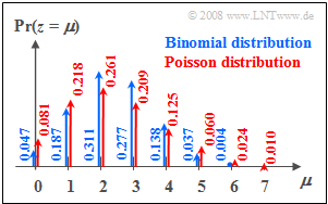
$\text{Example 1:}$ The probabilities
- of the binomial distribution with $I =6$, $p = 0.4$, and
- of the Poisson distribution with $λ = 2.4$
can be seen in the graph on the right. You can recognize:
- Both distributions have the same mean $m_1 = 2.4$.
- In the Poisson distribution (red arrows and labels) the "outer values" are more probable than in the binomial distribution.
- In addition, random variables $z > 6$ are also possible with the Poisson distribution, but their probabilities are also rather small at the chosen rate.
Moments of the Poisson distribution
$\text{Calculation rule:}$
- The »mean« and the »standard deviation« of the Poisson distribution are obtained directly from the $\text{corresponding equations of the binomial distribution}$ by twofold limiting:
- $$m_1 =\lim_{\left.{I\hspace{0.05cm}\to\hspace{0.05cm}\infty \atop {p\hspace{0.05cm}\to\hspace{0.05cm} 0} }\right.} I \cdot p= \lambda,$$
- $$\sigma =\lim_{\left.{I\hspace{0.05cm}\to\hspace{0.05cm}\infty \atop {p\hspace{0.05cm}\to\hspace{0.05cm} 0} }\right.} \sqrt{I \cdot p \cdot (1-p)} = \sqrt {\lambda}.$$
- From this it can be seen that in the Poisson distribution the variance is always $σ^2 = m_1 = λ$.
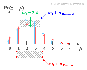
$\text{Example 2:}$
As in $\text{Example 1}$, here we compare:
- the binomial distribution with $I =6$, $p = 0.4$, and
- the Poisson distribution with $λ = 2.4$.
One can see from the accompanying sketch:
- Both distributions have exactly the same mean $m_1 = 2.4$.
- For the Poisson distribution (marked red in the figure), the standard deviation $σ ≈ 1.55$.
- In contrast, for the (blue) binomial distribution, the standard deviation is only $σ = 1.2$.
With the interactive HTML 5/JavaScript applet "Binomial and Poisson Distribution"
- you can determine the probabilities and means (moments) of the Poisson distribution for any $λ$-values
- and visualize the similarities and differences compared to the binomial distribution.
Comparison of binomial distribution vs. Poisson distribution
Now both the similarities and the differences between binomial and Poisson distributed random variables shall be worked out again.
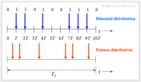
The »binomial distribution« is suitable for the description of such stochastic events, which are characterized by a given clock $T$. For example, for $\text{ISDN}$ ("Integrated Services Digital Network") with $64 \ \rm kbit/s$ ⇒ the clock time $T \approx 15.6 \ \rm µ s$.
- Binary events only occur in this time grid. Such events are, for example, error-free $(e_i = 0)$ or errored $(e_i = 1)$ transmission of individual symbols.
- The binomial distribution now allows statistical statements about the number of transmission errors to be expected in a longer time interval $T_{\rm I} = I ⋅ T$ according to the upper diagram of the graph (time marked in blue).
Also the »Poisson distribution« makes statements about the number of occurring binary events in a finite time interval:
- If one assumes the same observation period $T_{\rm I}$ and increases the number $I$ of subintervals more and more, then the clock time $T$, at which a new binary event ("0" or "1") can occur, becomes smaller and smaller. In the limiting case $T \to 0$.
- This means: In the Poisson distribution, the binary events are possible not only at discrete time points given by a time grid, but at any time. The time diagram below illustrates this fact.
- In order to obtain on average during time $T_{\rm I}$ exactly as many "ones" as in the binomial distribution (in the example: six), however, the characteristic probability $p = {\rm Pr}( e_i = 1)$ related to the infinitesimally small time interval $T$ must tend to zero.
Applications of the Poisson distribution
The Poisson distribution is the result of a so-called $\text{Poisson process}$. Such a process is often used as a model for sequences of events that may occur at random times. Examples of such events include.
- the failure of equipment - an important task in reliability theory,
- the shot noise in optical transmission, and
- the start of telephone calls in a switching center ("teletraffic engineering").
$\text{Example 3:}$ If ninety switching requests per minute $($⇒ $λ = 1.5 \text{ per second})$ are received by a switching center on a long–term average, the probabilities $p_\mu$ that exactly $\mu$ connections occur in any one-second period are:
- $$p_\mu = \frac{1.5^\mu}{\mu!}\cdot {\rm e}^{-1.5}.$$
This gives the numerical values $p_0 = 0.223$, $p_1 = 0.335$, $p_2 = 0.251$, etc.
From this, further characteristics can be derived:
- The distance $τ$ between two connection requests satisfies the $\text{exponential distribution}$.
- The mean time interval between two connection requests is ${\rm E}[\hspace{0.05cm}τ\hspace{0.05cm}] = 1/λ ≈ 0.667 \ \rm s$.
Exercises for the chapter
Exercise 2.5: "Binomial" or "Poisson"?


