Exercise 1.2Z: Lognormal Fading Revisited
From LNTwww
We assume similar conditions as in Exercise 1. 2 but now we summarize the purely distance-dependent path loss $V_0$ and the mean value $m_{\rm S}$ of the lognormal fading (the index "S" stands for Shadowing):
- $$V_{\rm 1} = V_{\rm 0} + m_{\rm S} \hspace{0.05cm}.$$
The total path loss is then given by the equation
- $$V_{\rm P} = V_{\rm 1} + V_{\rm 2}(t)$$
where $V_2(t)$ describes a lognormal distribution with mean value zero:
- $$f_{V_{\rm S}}(V_{\rm S}) = \frac {1}{ \sqrt{2 \pi }\cdot \sigma_{\rm S}} \cdot {\rm e }^{ - { (V_{\rm S}\hspace{0.05cm}- \hspace{0.05cm}m_{\rm S})^2}/(2 \hspace{0.05cm}\cdot \hspace{0.05cm}\sigma_{\rm S}^2) }\hspace{0.05cm}.$$
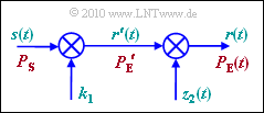
The path loss model shown in the graphic is suitable for the scenario described here:
- Multiply the transmitted signal $s(t)$ first with a constant factor $k_1$ and further with a stochastic quantity $z_2(t)$ with the probability density function $\rm (PDF)$ $f_{\rm z_2}(z_2)$.
- Then the signal $r(t)$ results at the output, whose power $P_{\rm E}(t)$ is of course also time-dependent due to the stochastic component.
- The PDF of the lognormally distributed random variable $z_2$ is for $z_2 ≥ 0$:
- $$f_{z_{\rm 2}}(z_{\rm 2}) = \frac {{\rm e^{- {\rm ln}^2 (z_{\rm 2}) /({2 \hspace{0.05cm}\cdot \hspace{0.05cm} C^2 \hspace{0.05cm} \cdot \hspace{0.05cm} \sigma_{\rm S}^2}) } } }{ \sqrt{2 \pi }\cdot C \cdot \sigma_{\rm S} \cdot z_2} \hspace{0.8cm}{\rm with} \hspace{0.8cm} C = \frac{{\rm ln} \hspace{0.1cm}(10)}{20\,\,{\rm dB}}\hspace{0.05cm}.$$
- For $z_2 ≤ 0$ this PDF is equal to zero.
Notes:
- This exercise belongs to the chapter Distance dependent attenuation and shading.
- Use the following parameters:
- $$V_{\rm 1} = 60\,{\rm dB}\hspace{0.05cm},\hspace{0.2cm} \sigma_{\rm S} = 6\,{\rm dB}\hspace{0.05cm}.$$
- The probability that a mean-free Gaussian random variable $z$ is greater than its standard deviation $\sigma$, is
- $${\rm Pr}(z > \sigma) = {\rm Pr}(z < -\sigma) = {\rm Q}(1) \approx 0.158\hspace{0.05cm}.$$
- Also, ${\rm Pr}(z > 2\sigma) = {\rm Pr}(z < -2\sigma) = {\rm Q}(2) \approx 0.023\hspace{0.05cm}.$
- Again for clarification: $z_2$ is the fading coefficient in linear units, while $V_2$ is the fading coefficient in logarithmic units.
- The following conversions apply:
- $$z_2 = 10^{-V_{\rm 2}/20\,{\rm dB}}\hspace{0.05cm}, \hspace{0.2cm} V_{\rm 2} = -20\,{\rm dB} \cdot {\rm lg}\hspace{0.15cm}z_2\hspace{0.05cm}.$$
Questions
Solution
(1) The constant $k_1$ generates the time-independent path loss $V_1 = 60 \ \rm dB$. From this follows:
- $$k_{\rm 1} = 10^{-V_{\rm 1}/(20\hspace{0.05cm} {\rm dB})} \hspace{0.15cm} \underline{= 0.001}\hspace{0.05cm}.$$
(2) Only the second statement is correct:
- For the Gaussian random variable $V_2$ all values between $-∞$ and $+∞$ are (theoretically) possible.
- The transformation $z_2 = 10^{{\it -V_2}\rm /20}$ results in only positive values for the linear random variable $z_2$,
namely between 0 $($if $V_2$ is positive and goes to infinity$)$ and $+∞$ $($very large negative values of $V_2)$.
(3) The random value $z_2$ can only be positive. Therefore the PDF value $f_{\rm z2}(z_2 = 0)\hspace{0.15cm}\underline{= 0}$.
- The PDF–value for the abscissa value $z_2 = 1$ is obtained by inserting it into the given equation:
- $$f_{z{\rm 2}}(z_{\rm 2} = 1) \hspace{-0.1cm} \ = \ \hspace{-0.1cm} \frac {{\rm e^{- {\rm ln}^2 (z_{\rm 2}=1) /({2 \hspace{0.05cm}\cdot \hspace{0.05cm} C^2 \hspace{0.05cm} \cdot \hspace{0.05cm} \sigma_{\rm S}^2}) } } }{ \sqrt{2 \pi }\cdot C \cdot \sigma_{\rm S} \cdot (z_2 = 1)} = \frac {1}{ \sqrt{2 \pi } \cdot 6\,\,{\rm dB} } \cdot \frac {20\,\,{\rm dB}}{ {\rm ln} \hspace{0.1cm}(10) } \hspace{0.15cm} \underline{\approx 0.578}\hspace{0.05cm}.$$
- The first portion is equal to the PDF–value $f_{V2}(V_2 = 0)$.
- $C$ considers the magnitude of the derivative of the non-linear characteristic $z_2 = g(V_2)$ for $V_2 = 0 \ \rm dB$ or $z_2 = 1$.
- Finally, for $z_2 = 2$:
- $$f_{z{\rm 2}}(z_{\rm 2} = 2) \hspace{-0.1cm} \ = \ \hspace{-0.1cm} \frac {f_{z{\rm 2}}(z_{\rm 2} = 1)}{ z_{\rm 2} = 2} \cdot {\rm exp } \left [ - \frac {{\rm ln}^2 (2)}{2 \cdot C^2 \cdot \sigma_{\rm S}^2} \right ]= \frac {0.578}{ 2} \cdot {\rm exp } \left [ - \frac {0.48}{0.952} \right ] \hspace{0.15cm} \underline{\approx 0.174}\hspace{0.05cm}. $$
(4) If you take into account the relationship between $z_2$ and $V_2$, you get
- $${\rm Pr}(z_{\rm 2} > 1) \hspace{-0.1cm} \ = \ \hspace{-0.1cm} {\rm Pr}(V_{\rm 2} < 0\,\,{\rm dB})\hspace{0.15cm} \underline{= 0.5} \hspace{0.05cm},$$
- $${\rm Pr}(z_{\rm 2} > 0.5) \hspace{-0.1cm} \ = \ \hspace{-0.1cm} {\rm Pr}(V_{\rm 2} < 6\,\,{\rm dB}) = 1- {\rm Pr}(V_{\rm 2} > 6\,\,{\rm dB})= 1- {\rm Pr}(V_{\rm 2} > \sigma_{\rm S})= 1- {\rm Q}(1)\hspace{0.15cm} \underline{= 0.842} \hspace{0.05cm},$$
- $${\rm Pr}(z_{\rm 2} > 4) \hspace{-0.1cm} \ = \ \hspace{-0.1cm} {\rm Pr}(V_{\rm 2} < -12\,\,{\rm dB}) = {\rm Pr}(V_{\rm 2} > +12\,\,{\rm dB}) = {\rm Pr}(V_{\rm 2} > 2 \sigma_{\rm S}) \hspace{0.05cm}.$$
- The probability that a Gaussian variable is greater than $2 \cdot \sigma$ equals ${\rm Q}(2)$:
- $${\rm Pr}(z_{\rm 2} > 4) = {\rm Q}(2)\hspace{0.15cm} \underline{= 0.023} \hspace{0.05cm}.$$
(5) The statement 3 is correct:
- The first statement is certainly not correct, since the mean value $m_{\rm S}$ refers to the logarithmic received power $($in $\rm dBm)$.
- To clarify whether the second or the third statement is correct, we assume $P_{\rm S} = 1 \ \rm W$, $V_1 = 60 \ \rm dB$ ⇒ $P_{\rm E}' = 1 \ {\rm µ W}$ and the following PDF for $V_2$:
- $$f_{V{\rm 2}}(V_{\rm 2}) = 0.5 \cdot \delta (V_{\rm 2}) + 0.25 \cdot \delta (V_{\rm 2}- 10\,\,{\rm dB}) + 0.25 \cdot \delta (V_{\rm 2}+ 10\,\,{\rm dB})\hspace{0.05cm}.$$
- Half of the time, $P_{\rm E} = 1 \ \rm µ W$, while each of the following has $25\%$ probability::
- $$V_{\rm 2}= +10\,\,{\rm dB}\text{:} \hspace{0.3cm} P_{\rm E}(t) \hspace{-0.1cm} \ = \ \hspace{-0.1cm} \frac{1\,\,{\rm W}}{10^7} = 0.1\,\,{\,}{\rm µ W}\hspace{0.05cm},$$
- $$V_{\rm 2}= -10\,\,{\,}{\rm dB}\text{:} \hspace{0.3cm} P_{\rm E}(t) \hspace{-0.1cm} \ = \ \hspace{-0.1cm} \frac{1\,\,{\rm W}}{10^5} = 10\,\,{\,}{\rm µ W}\hspace{0.05cm}.$$
- The mean value is then:
- $${\rm E}[P_{\rm E}(t)] = 0.5 \cdot 1\,{\rm µ W}+ 0.25 \cdot 0.1\,{\rm µ W}+ 0.25 \cdot 10\,{\rm µ W}= 3.025\,{\rm µ W} > P_{\rm E}\hspace{0.05cm}' = 1\,{\rm µ W} \hspace{0.05cm}.$$
- This simple calculation with discrete probabilities instead of a continuous PDF indicates that statement 3 is correct.
