Possible Errors when using DFT

The Mean Square Error As a Quality Criteria

In the following, we briefly discuss some error possibilities when applying the DFT, whereby we restrict ourselves to the transformation from the time to the frequency domain. Even in its samples, the spectrum $D(\mu )/f_{\rm A}$ determined via the DFT will generally differ from the actual spectrum $X(\mu \cdot f_{\rm A})$ due to two processes:

the sampling, that is, the reduction of information about $x(t)$ to $N$ numerical values,
the windowing that limits the signal $x(t)$ possibly erroneously.

$\text{Definition:}$ A quality criteria that takes both types of error into account is the mean square error:

$${\rm MQF} = \frac{1}{N}\cdot \sum_{\mu = 0 }^{N-1} \left\vert X(\mu \cdot f_{\rm A})-\frac{D(\mu)}{f_{\rm A} }\right \vert^2 \hspace{0.05cm}.$$

It is always ${\rm MQF} \ne 0$, since with finite $N$ degradation due to sampling and due to windowing cannot be made zero at the same time

.

The magnitude of this evaluation quantity ${\rm MQF}$ depends on the following parameters:

the properties of the time function at hand $x(t)$ or the spectrum $X(f)$,
the DFT parameter $N$; the larger $N$ is chosen, the smaller ${\rm MQF}$ becomes,
one of the four further DFT parameters, for example $f_{\rm A}$.

For a given $N$ the other DFT parameters are determined via the equations $f_{\rm P} = N \cdot f_{\rm A}$, $T_{\rm P} = 1/f_{\rm A}$ and $T_{\rm A} = T_{\rm P}/N$ .

We refer you already here to the learning video (in German language) Possible Errors When Using DFT , which clarifies the content of this chapter.

Quasi-Error-Free DFT with $N = 16$

$\text{Example 1:}$ As an example, we consider a Gaussian pulse with the equivalent pulse duration $\Delta t = T$, where $T$ is simultaneously used as a normalisation parameter:

$$x(t) = {\rm e}^{- \pi (t/T)^2} \hspace{0.05cm}.$$

The Gaussian pulse is very suitable for the application of DFT due to its fast, exponential decay in both the time and frequency domain.

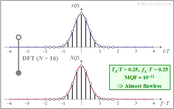
The graph below shows the DFT–result

for $N = 16$ and
$T_{\rm A}/T = 0.25$ ⇒ $f_{\rm A} \cdot T = 0.25$.

The following should be noted about this plot:

The considered samples of $x(t)$ are in the range $\vert t/T \vert≤ 2$. Since $x(\pm 2T)$ is very small, periodization in the time domain with $T_{\rm P}/T = N \cdot T_{\rm A}/T = 2$ does not lead to serious errors.
With $f_{\rm A} \cdot T = 0.25$ and $N = 16$ results in the (normalised) DFT parameter $f_{\rm P} \cdot T = 4$.
The discrete spectral lines of the DFT thus lie in the range $-2/T ≤ f < +2/T$.
The mean squared error is relatively small $\text{(MQF} \approx 10^{-12})$, which is due to the favourable choice of $f_{\rm A} \cdot T = 0.25$ $($for a given $N = 16)$ .
The DFT accuracy can be improved by increasing $N$ :

For $N = 1024$ the smallest possible value is obtained $\text{MQF} \approx 8 \cdot 10^{-17}$, if $f_{\rm A} \cdot T = 0.125$ is chosen. The following then applies to the other DFT parameters:

$$f_{\rm P} \cdot T = 128, \hspace{0.5cm}T_{\rm A}/T = 1/128, \hspace{0.5cm} T_{\rm P}/T = N \cdot T_{\rm A}/T= 8.$$

For a 32–bit–processor (meaning: smaller quantization errors of the computer) $\text{MQF}$ would be even smaller, but never zero.

DFT Falsification Due to Windowing – Termination Error

A typical error when using the DFT is due to windowing' . This falsification, known as truncation error can be explained as follows:

The windowing implicit in the DFT algorithm corresponds to the multiplication of the signal $x(t)$ by a rectangular function of height $1$ and duration $T_{\rm P} = N \cdot T_{\rm A}$.
If the time signal $x(t)$ is not limited to the range $T_{\rm P}$ the DFT result does not coincide with the actual spectrum $X(f)$ but is obtained from it by convolution with the spectral function $T_{\rm P} \cdot \text{si}(\pi fT_{\rm P})$.
In the limiting case $T_{\rm P} \to \infty$, which for a given distance $T_{\rm A}$ of the samples would also mean an infinitely large number of interpolation points $N$ degenerates $T_{\rm P} \cdot \text{si}(\pi fT_{\rm P})$ to a Dirac function and the original spectrum $X(f)$ would remain.
The DFT of an unbounded signal in time - for example a periodic signal - will always cause a truncation error which can only be kept within limits by special measures. This is discussed in more detail in the chapter spectrum analysis .
For time-limited, pulse-like signals, the truncation error can be avoided by choosing $T_{\rm P}$ sufficiently large. By further enlarging the window into areas with $x(t) \approx 0$ no additional information gain results ⇒ $\text{MQF}$ does not become smaller.
By this addition of zeros (zero-padding) the samples of $X(f)$ now occur at a smaller distance $f_{\rm A} = 1/T_{\rm A}$ . By $T_{\rm P}$-doubling one achieves an interpolation of the frequency samples exactly in the middle between two previous grid points.

The following example shows a termination error due to unfavourably chosen DFT parameters.

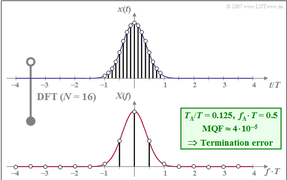
Termination Error For a DFT With $N = 16$

$\text{Example 2:}$ The graph shows the result of the DFT for equal $x(t)$ and $X(f)$ as well as equal $N = 16$ as in $\text{example 1}$,but now with sampling in the time domain finer by a factor of $2$ compared to this:

$$T_{\rm A}/T = 0.125 ⇒ f_{\rm A} \cdot T = 0.5.$$

The comparison with example 1 $(T_{\rm A}/T = 0.25 \ \Rightarrow \ f_{\rm A} \cdot T = 0.25)$ shows:

The spacing of the frequency samples increases: $f_{\rm A} \cdot T = 0.5$.
At the same time, $T_{\rm P}/T$ decreases from $4$ to $2$.
With this, only the signal components in the range $\vert t \vert < T$ are now captured by the DFT.

Summing up:
With these DFT parameters, a truncation error arises, by which the mean square error $\rm (MQF)$ is significantly increased from $10^{-12}$ to $4 \cdot 10^{-5}$ .

Again, we refer to the learning video (in German language)
Possible Errors When Using DFT.

DFT Falsification Due To Sampling – Aliasing Error

An unsuitable sampling of the time function $x(t)$ can also significantly falsify the DFT result. This so-called aliasing error can be explained as follows:

Sampling $x(t)$ at a distance $T_{\rm A}$ causes a periodic continuation of the spectrum at multiples of the periodisation frequency $f_{\rm P} = 1/T_{\rm A}$.
If the spectrum $X(f)$ also has spectral components at $|f| > f_{\rm P}/2$, the sampling theorem is not fulfilled and overlaps of the shifted frequency components to be added occur.
Only with a band-limited signal can the aliasing error be avoided by suitable DFT parameters. In contrast, this error is unavoidable with time-limited, pulse-like signals, since time-limited signals cannot be band-limited at the same time.
The aliasing error is reduced by finer sampling $($so: smaller $T_{\rm A} = 1/f_{\rm P})$ . This can only be achieved with a constant $T_{\rm A}$ - in order not to let the truncation error increase - by a larger $N$ and thus a greater computational effort.

The following $\text{Example 3}$ shows such an aliasing error due to wrongly chosen DFT parameters:

Compared to the „comparison system” according to $\text{example 1}$ is $T_{\rm A}$ too large and $f_{\rm A}$ too small dimensioned.
The number of interpolation points is in both cases $N = 16$.

Aliasing Error of a DFT With $N = 16$

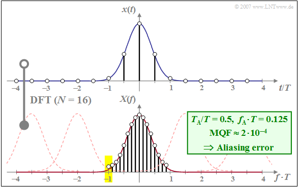
$\text{Example 3:}$ Let the DFT parameters be $N = 16$ and $f_{\rm A} \cdot T= 0.125$. Thus, for the other three DFT parameters we get:

$T_{\rm P}/T = 8.0 \hspace{0.5cm} \text{(Example 1:} \ \ T_{\rm P}/T = 4)$,
$f_{\rm P} \cdot T = 2.0 \hspace{0.45cm} \text{(Example 1:} \ \ f_{\rm P} \cdot T = 4)$,
$T_{\rm A}/T = 0.5\hspace{0.45cm} \text{(Example 1:} \ \ T_{\rm A}/T = 0.25)$.

This results in the following consequences:

The termination error continues to play no role because of $T_{\rm P} /T = 8$ (already $T_{\rm P} /T = 4$ was sufficient).
Because $f_{\rm P} \cdot T = 2$ aliasing now arises, however, because the DFT is derived from the sum of many Gaussian functions at distance $f_{\rm P} \cdot T = 2$ (thin dashed curves in the graph ).
The individual DFT coefficients are falsified differently: The mean DFT coefficient $($for the frequency $f = 0)$ is almost correct, while the errors of the DFT coefficients increase significantly towards the edges.
In the example considered, the DFT coefficient for $f \cdot T = -1$ is twice as large as it should be, since the Gaussian function with the centre at $f \cdot T = -2$ gives the same contribution as the actual Gaussian function around $f \cdot T = 0$ (see yellow background).

Thus, here with $\text{MQF} \approx 2 \cdot 10^{-4}$ an error value four times larger than that caused by the termination error in $\text{example 2}$.

Again, we refer to the learning video (in German language) Possible Errors When Using DFT.

Exercises For The Chapter

Exercise 5.3: Mean Square Error

Exercise 5.3Z: Zero-Padding

Possible Errors when using DFT

Contents

The Mean Square Error As a Quality Criteria

DFT Falsification Due to Windowing – Termination Error

DFT Falsification Due To Sampling – Aliasing Error

Exercises For The Chapter