Spectrum Analysis

Spectral leakage effect

$\text{Definition:}$ The term »spectral leakage effect« is used to describe the distortion of the spectrum of a periodic and thus temporally unlimited signal due to the implicit time limit of the »Discrete Fourier Transform« $\rm (DFT)$. This means that, for example, a spectrum analyzer

fake frequency components that are not present in the time signal, and/or

actually existing spectral components are hidden by side lobes.

The following $\text{Example 1}$ will show that for a periodic signal the application of the »Discrete Fourier Transform« $\text{(DFT)}$ is not useful without additional measures. The quality of the spectral analysis – i.e. the correctness of the spectrum found – is mainly determined here by the $($more or less successful$)$ adaptation of the DFT parameters to the signal parameters at hand.

If the period $T_0$ of the signal is known, the duration $T_{\rm P}$ of the signal section used for the DFT should be an integer multiple of $T_0$.
However, the task of spectral analysis is precisely to find arbitrary signal components, so that the knowledge of $T_0$ cannot generally be assumed.
A measure to improve the spectral analysis is the windowing with a suitable time function $w(t)$. The product signal $x(t) \cdot w(t)$ is then analyzed.
A large number of such window functions $w(t)$ are known from the literature, which lead to good or less satisfactory results depending on the task.

In the next sections the spectral leakage effect will be illustrated by examples and the advantages and disadvantages of the different window functions will be discussed. So much up front: There is no "best" window function for all applications.

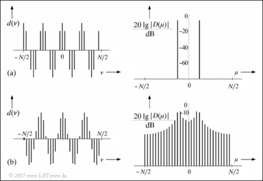
$\text{Example 1:}$ The upper graph (a) from [Söd93]^[1] shows the discrete-time signal $d(\nu)$ of a harmonic oscillation with frequency $f_0 = 125\,\text{ kHz}$ ⇒ period duration $T_0 = 8 \,{\rm µ s}$. The distance between two successive time samples in this example is chosen to be $T_{\rm A} = 1 \,{\rm µ s}$ .

Example of applying spectral analysis

⇒ On the right the frequency discrete spectrum $\vert D(\mu) \vert$ after a DFT with $N = 32$ samples is shown in logarithmic form (in dB), from which the further DFT parameters result as follows:

Duration of the time segment: $T_{\rm P} = 32 \,{\rm µ s}$,

gridding of the frequency axis: $f_{\rm A} = 31.25 \,\text{ kHz}$.

Since the interval width $T_{\rm P}$ captures an integer multiple of period $T_0$, the DFT delivers the correct result. The two Dirac delta functions lie exactly at $\pm4 \cdot f_{\rm A}$.

⇒ If one measures an oscillation of frequency $f_0 = 109.375\,\text{ kHz}$ ⇒ period $T_0 = 9.14 \,{\rm µ s}$ corresponding to the graph below (b), significant distortions of the spectrum occur.

Since now $T_{\rm P}/T_0 = 3.5$ is no longer an integer, the periodic continuation of the time section causes phase jumps, in our example by $\pi$.

The spectral range now no longer consists of two Dirac delta functions as in the sketch (a), but of an approximately continuous frequency function with the maximum near the actual signal frequency and a series of further parts, which are called »side lobes«.

Describing windowing from a system theory perspective

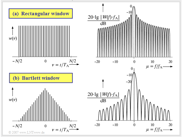
The occurrence of such unwanted side lobes is now to be explained using the following diagram. This graphic was also taken from the book [Söd93]^[1]

Rectangular window $($top$)$ and Bartlett window $($bottom$)$

First consider the upper graph (a) for the »rectangular window«.

The time limit implicit in the DFT corresponds to the multiplication of the signal $x(t)$ by a rectangular window function $w(t)$ of height $1$ and duration $T_{\rm P}$.

The upper left graph shows the discrete-time representation of this rectangular function with the normalized time variable $\nu= t/T_{\rm A}$:

$${w} (\nu) = \left\{ \begin{array}{c} 1 \\ 0 \\ \end{array} \right.\quad \begin{array}{*{10}c} {\rm{for}} \\ \\ \end{array}\begin{array}{*{20}c} -N/2 \le \nu < N/2 \hspace{0.05cm}, \\ {\rm else} \hspace{0.05cm}. \\ \end{array}$$

From the multiplication $y(t) = x(t) \cdot w(t)$ of the signal $x(t)$ to be analyzed and the window function $w(t)$ follows for the spectral function $Y(f) = X(f) \ast W(f)$, where for the rectangular window with $f_{\rm A} = 1/T_{\rm P}$ and ${\rm si}(x) = \sin(x)/x = {\rm sinc}(x/\pi) $ holds:

$$W(f) = T_{\rm P} \cdot {\rm sinc}(f \cdot T_{\rm P}) = {1}/{f_{\rm A}}\cdot {\rm sinc}({f}/{f_{\rm A}})\hspace{0.05cm}.$$

The spectral function $W(f)$ is shown logarithmically in the upper right graph. If all spectral components of $x(t)$ lie in the frequency grid $\mu \cdot f_{\rm A}$, the discrete frequency spectral values $D(\mu )$ remain unchanged by the convolution with $W(f)$.

Otherwise, convolution with $W(f)$ leads to distortions, since the zeros of the $\rm sinc$ function no longer fit the discrete values of the input spectrum.

The discontinuities in the time domain caused by limitation and periodic continuation are reduced if, instead of the constant one weighting by the rectangle, the two edge areas of the window are weighted weaker than the center.

Consider the graph (b) for the »Bartlett window« – also called "triangular window":

The discrete-time description of the Bartlett window is with $\nu = t/T_{\rm A}$:

$${w} (\nu) = \left\{ \begin{array}{c} 1 - {2 \hspace{0.05cm} \cdot \hspace{0.05cm} |\nu|}/{N} \\ 0 \\ \end{array} \right.\quad \begin{array}{*{10}c} {\rm{for}} \\ \\ \end{array}\begin{array}{*{20}c} -N/2 \le \nu < N/2 \hspace{0.05cm}, \\ {\rm else} \hspace{0.05cm}. \\ \end{array}$$

From this follows for the continuous-time window function $w(t)$ and the spectral representation $W(f)$:

$${w} (t) = \left\{ \begin{array}{c} 1 -{|t|}/{(T_{\rm P}/2)} \\ 0 \\ \end{array} \right.\hspace{0.05cm} \begin{array}{*{20}c} |t| \le T_{\rm P}/2\\ {\rm else} \\ \end{array}\hspace{0.2cm}\circ\!\!-\!\!\!-\!\!\!-\!\!\bullet\, \hspace{0.2cm}W(f) ={1}/({2f_{\rm A}})\cdot {\rm sinc}^2( {f}/({2f_{\rm A}}))\hspace{0.05cm}.$$

Due to the lower weighting of the edge regions, which are particularly problematic with unbounded signals, the $($logarithmically drawn$)$ spectrum $W(f)$ has lower side lobes than the $\rm sinc$ function in the upper graph, which leads to lower leakage components.

The better suppression of the side lobes, however, comes at the cost of a noticeable reduction and broadening of the main lobe, limiting the resolving power of the Bartlett window compared to rectangular windowing.

Special window functions

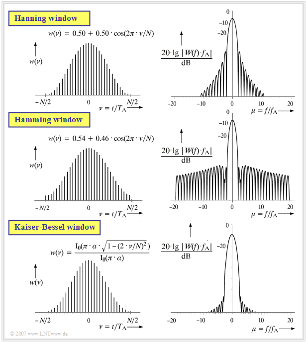
Hanning window, Hamming window and Kaiser-Bessel window

Now some frequently used »window functions«, viz.

the Hanning window,

the Hamming window, and

the Kaiser-Bessel window

will be described by means of graphs and equations contained therein.

For the running variable in the time domain always applies:

$$-N/2 ≤ \nu < N/2.$$

Notes:

In the Kaiser-Bessel window, the functions in the time and frequency domain are each shown for $\alpha = 3.5$.

${\rm I}_0(.)$ denotes the »modified zero-order Bessel function«.

Further window functions such as the »Blackman-Harris window», the »cosine rolloff window« $($also called Tukey window$)$ and many more can be found in the book [Söd93]^[1].

The suitability of these window functions for various tasks of spectral analysis is mentioned in the next section.

Quality criteria of window functions

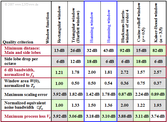
The table shows quality criteria for the window functions described in the last sections. The selection of a suitable window function should be made according to the following aspects:

Compilation of important quality criteria of window functions

Illustrating the »6dB bandwidth«

The »minimum distance between main lobe and side lobes« should be as large as possible to keep the influence of the leakage effect low and to improve the amplitude resolution.

For reasons of good frequency selectivity, the »6dB bandwidth« should be small. If this parameter is too large, a dominant spectral line will mask smaller components in the surrounding area.

The »maximum process loss« includes the maximum scaling error and the equivalent noise bandwidth. This value should never exceed $\text{3.7 dB}$.

These three most important quality criteria are highlighted in red in the adjacent table.

In each row, rather favourable window functions are highlighted in green and rather unfavourable ones in grey.
From the distribution of the green and grey areas it is already evident that the optimal window function does not exist.

Now the quality criteria given in the table are described in more detail:

The larger the »minimum main-to-side lobe distance« ⇒ ratio of the main lobe to the highest side lobe, the better the amplitude resolution of a window function.

As expected, for the rectangle this distance is smallest $\text{(13 dB)}$. The best result $\text{(92 dB)}$ is achieved with the fourth-order Blackman-Harris window.

However, since not only the highest but also all other side lobes contribute to the leakage effect, the »side lobe drop« is another measure for the resolving power.

Of the given window functions, the Hanning window and the cosine rolloff window with rolloff $r = 0.5$ have the most favourable values in this respect $\text{(18 dB/octave)}$.

The »6 dB bandwidth«, which can be read from the logarithmized spectral function, is an important measure of frequency resolving.

Two spectral components in the signal at $f_1$ and $f_2$ can only be resolved if the difference $f_2 - f_1$ is greater than the »6dB bandwidth« of the window function used $($see lower graph$)$.

The »window area« of the function $w(t)$ at the same time gives the height $W(0)$ in the spectral domain.

For all windows except the rectangle, $W(0)<1$ and thus a DFT amplitude error results due to the suppression of outer samples, which, however, can be completely corrected if $w(t)$ is known.

Maximum process loss

This combined quality criterion considers

the »maximum scaling error« as well as

the (normalized) »equivalent noise bandwidth«.

The maximum process loss is usually given in $\text{dB}$ and should be $($according to its name$)$ rather small:

$$10 \cdot {\rm lg}\hspace{0.15cm}V_{\rm P}\hspace{0.15cm}{\rm (in}\hspace{0.15cm}{\rm dB)}= 20 \cdot {\rm lg}\hspace{0.15cm} \frac{|W(f=0)|}{|W(f=f_{\rm A}/2)|} + 10 \cdot {\rm lg}\hspace{0.15cm} \frac{\int_{-\infty}^{\infty}|W(f)|^2\hspace{0.05cm}{\rm d}f}{f_{\rm A} \cdot |W(f=0)|^2} \hspace{0.05cm}.$$

From the »table in the last section« it can be seen that for the window functions considered $V_{\rm P}$ takes values between $\text{3 dB}$ and $\text{4 dB}$, where window functions with $V_{\rm P} > 3. 7 \,\text{dB}$ $($rectangle, Blackman-Harris, Kaiser-Bessel$)$ should not be used. However, it is precisely these that are best with regard to the main-to-side lobe distance.

The two proportions are to be interpreted as follows:

The »maximum scaling error« is the ratio by which the amplitude determined with the DFT differs from the actual signal amplitude. Hereby, the amplitude error due to a window area smaller than $1$ is assumed to be corrected.
The wider the main lobe of the window function, the smaller this scaling error. The error is largest when the frequency $f_0$ of a harmonic oscillation lies midway between two DFT support points ⇒ quotient $|W(f = 0)| / |W(f = f_{\rm A}/2)|$.
The »equivalent noise bandwidth« of the window function is calculable as the width of the equal-area rectangle with respect to the magnitude square $|W(f)|^2$ of the spectral function. This parameter captures the disturbing influence of white noise and should be as small as possible.
The smallest noise bandwidth results for the rectangle. All other window functions have a larger noise bandwidth and thus, in the presence of noise, also a $($significantly$)$ less favourable signal-to-noise power ratio.

$\text{The results of this section can be summarized as follows:}$

An ideal window function does not exist. Depending on the task $($good amplitude or frequency resolution$)$ different windows provide the best result in each case. It is therefore recommended that one always uses several window functions for spectral analysis or at least one window function with different parameters.

A workable compromise with regard to all criteria is the »Hamming window« which only gives one unfavourable value $($»side lobe drop« only 6 dB per octave$)$.

Although the »Hanning window« differs only marginally from the Hamming window in the time domain, in the spectral domain $($»minimum distance between main lobe and side lobes«) the difference between these two windows is considerable.

Exercises for the chapter

Exercise 5.4: Comparison of Rectangular and Hanning Window

Exercise 5.4Z: On the Hanning Window

References

↑ ^1.0 ^1.1 ^1.2 Söder, G.: Modellierung, Simulation und Optimierung von Nachrichtensystemen. In: Berlin – Heidelberg: Springer, 1993.

[S.C3.B6d93-1] 1.0 ^1.1 ^1.2 Söder, G.: Modellierung, Simulation und Optimierung von Nachrichtensystemen. In: Berlin – Heidelberg: Springer, 1993.

[1]