The Convolution Theorem and Operation

Convolution in the time domain

The "Convolution Theorem" is one of the most important laws of the Fourier transform, to which an own subchapter is dedicated in this tutorial.

We will first consider the convolution theorem in the time domain and assume that the spectra of two time functions $x_1(t)$ and $x_2(t)$ are known:

$$X_1 ( f )\hspace{0.15cm}\bullet\!\!\!-\!\!\!-\!\!\!-\!\!\circ\hspace{0.15cm}x_1( t ),\quad X_2 ( f )\hspace{0.1cm}\bullet\!\!\!-\!\!\!-\!\!\!-\!\!\circ\hspace{0.1cm}x_2 ( t ).$$

Then for the time function of the product $X_1(f) \cdot X_2(f)$ applies:

$$X_1 ( f ) \cdot X_2 ( f )\hspace{0.15cm}\bullet\!\!\!-\!\!\!-\!\!\!-\!\!\circ\hspace{0.15cm}\int_{ - \infty }^{ + \infty } {x_1 ( \tau )} \cdot x_2 ( {t - \tau } )\hspace{0.1cm}{\rm d}\tau.$$

Here $\tau$ is a formal integration variable with the dimension of a time.

$\text{Definition:}$ The above connection of the time function $x_1(t)$ and $x_2(t)$ is called $\text{convolution}$ and represents this functional connection with a star:

$$x_{\rm{1} } (t) * x_{\rm{2} } (t) = \int_{ - \infty }^{ + \infty } {x_1 ( \tau ) } \cdot x_2 ( {t - \tau } ) \hspace{0.1cm}{\rm d}\tau = x_{\rm{2} } (t) * x_{\rm{1} } (t) .$$

Thus the above Fourier correspondence can be written as follows:

$$X_1 ( f ) \cdot X_2 ( f )\hspace{0.15cm}\bullet\!\!\!-\!\!\!-\!\!\!-\!\!\circ\hspace{0.15cm}{ {x} }_{\rm{1} } ( t ) * { {x} }_{\rm{2} } (t ).$$

The convolution is $\text{"commutative"}$ ⇒ The order of the operands can be changed:

$$x_1(t) * x_2(t) =x_2(t) * x_1(t).$$

The Proof will be shown at the end of the chapter.

On calculation of signal and spectrum of the LTI output

$\text{Example 1:}$ Every linear time-invariant $\rm (LTI)$ system can be described both,

by the frequency response $H(f)$,
by the impulse response $h(t)$.

The relation between these two system quantities is also given by the Fourier transform.

If a signal $x(t)$ with spectrum $X(f)$ is applied to the input, the spectrum of the output signal is:

$$Y(f) = X(f) \cdot H(f)\hspace{0.05cm}.$$

It is possible to calculate the output signal in the time domain with the convolution theorem:

$$y( t ) = x(t) * h( t ) = \int_{ - \infty }^{ + \infty } \hspace{-0.15cm}{x( \tau )} \cdot h( {t - \tau } )\hspace{0.1cm}{\rm d}\tau = \int_{ - \infty }^{ + \infty } \hspace{-0.15cm} {h( \tau )} \cdot x( {t - \tau } )\hspace{0.1cm}{\rm d}\tau = h(t) * x( t ).$$

This equation shows again the "commutativity" of the convolution operation.

Convolution in the frequency domain

The duality between time and frequency domain also allows statements regarding the spectrum of the product signal:

$$x_1 ( t ) \cdot x_2 ( t )\circ\!\!-\!\!\!-\!\!\!-\!\!\bullet\,X_1 (f) * X_2 (f) = \int_{ - \infty }^{ + \infty } {X_1 ( \nu )} \cdot X_2 ( {f - \nu })\hspace{0.1cm}{\rm d}\nu.$$

This result can be proved similarly to the "Convolution in the Time Domain". However, the integration variable $\nu$ now has the dimension of a frequency.

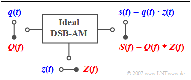
Convolution in the frequency domain (e.g. DSB–AM)

$\text{Example 2:}$ The Double-Sideband Amplitude Modulation $\text{(DSB-AM)}$ with carrier suppression is described by the drawn model.

The time domain representation $\rm (blue)$ shows the modulated signal $s(t)$ as the product of the source signal $q(t)$ and the (normalized) carrier signal $z(t)$.

According to the convolution theorem it follows for the frequency domain $\rm (red)$ that the output spectrum $S(f)$ is equal to the convolution product of $Q(f)\ \bullet\!\!-\!\!\!-\!\!\!-\!\!\circ \ q(t)$ and $Z(f)\ \bullet\!\!-\!\!\!-\!\!\!-\!\!\circ \ z(t)$.

Convolution of a function with a Dirac function

The convolution operation becomes very simple, if one of the two operands is a Dirac function. This applies equally to the convolution in the time and frequency domain.

We will consider the convolution of a function $x_1(t)$ with the function

$$x_2 ( t ) = \alpha \cdot \delta ( {t - T} ) \quad \circ\,\!\!\!-\!\!\!-\!\!\!-\!\!\bullet \quad X_2 ( f )= \alpha \cdot {\rm{e}}^{ - {\rm{j}}\hspace{0.05cm}\cdot\hspace{0.05cm}2\hspace{0.03cm}{\rm{\pi }}\hspace{0.05cm}\cdot\hspace{0.05cm}f\hspace{0.05cm}\cdot\hspace{0.05cm}T}.$$

For the spectral function of the signal $y(t) = x_1(t) \ast x_2(t)$ it follows:

$$Y( f ) = X_1 ( f ) \cdot X_2 ( f ) = X_1 ( f ) \cdot \alpha \cdot {\rm{e}}^{ - {\rm{j}}\hspace{0.05cm}\cdot\hspace{0.05cm}2\hspace{0.03cm}{\rm{\pi }}\hspace{0.05cm}\cdot\hspace{0.05cm}f\hspace{0.05cm}\cdot\hspace{0.05cm}T}.$$

The complex exponential function leads to a shift by $T$ ⇒ Shifting Theorem, the factor $\alpha$ to a damping $(\alpha < 1)$ or amplification $(\alpha > 1)$.

From this follows:

$$x_1 (t) * x_2 (t) = \alpha \cdot x_1 ( {t - T} ).$$

$\text{In Words: }$

The convolution of any function with a Dirac function at $t = T$ results in the function shifted to the right by $T$,
while the weighting of the Dirac function by the factor $\alpha$ has to be taken into account.

Convolution of a rectangle pulse with a Dirac function

$\text{Example 3:}$ A rectangle pulse $x(t)$ is delayed by an LTI system by the delay time $\tau = 3\,\text{ ms}$ and attenuated by the factor $\alpha = 0.5$ .

Shift and damping can be recognised both

by the output signal $y(t)$
as well as from the impulse response $h(t)$.

Graphical convolution

For the descriptions on this page the following convolution operation is assumed:

Screenshot of an older version of the $\rm LNTwww$ applet "Convolution":
$x_1(t)$ is denoted as $x(t)$ and $x_2(t)$ as $h(t)$

$$y(t) = x_1 (t) * x_2 (t) $$

$$\Rightarrow \hspace{0.3cm}y(t) = \int_{ - \infty }^{ + \infty } {x_1 ( \tau )} \cdot x_2 ( {t - \tau } )\hspace{0.1cm}{\rm d}\tau.$$

The solution of the convolution integral shall be done graphically. It is assumed that $x_1(t)$ and $x_2(t)$ are continuous time signals.

Then the following steps are required:

Change time variables of the functions: $x_1(t) \to x_1(\tau)$, $x_2(t) \to x_2(\tau)$.
Mirroring the second function: $x_2(\tau) \to x_2(-\tau)$.
Shifting the mirrorred function by $t$: $x_2(-\tau) \to x_2(t-\tau)$.
Multiplication of both functions $x_1(\tau)$ and $x_2(t-\tau)$.
Integration over the product respective $\tau$ between the limits $-\infty$ to $+\infty$.

Since the convolution is commutative, $x_1(\tau)$ can also be mirrored instead of $x_2(\tau)$.

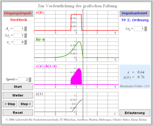
The topic is illustrated by the (newer) HTML5 applet Graphical Convolution.

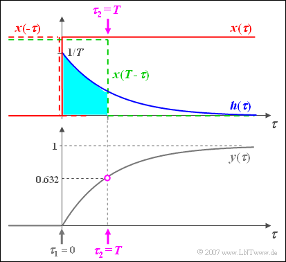
Jump function convoluted with the exponential function

$\text{Example 4:}$ The procedure for the graphical convolution is now explained with a detailed example:

At the input of a filter there is a jump function $x(t) = \gamma(t)$.
The impulse response of the first order low-pass filter is $h( t ) = {1}/{T} \cdot {\rm{e} }^{ - t/T}.$
The time axis is already renamed to $\tau$.

The graphic shows

the (red colored) input signal $x(\tau)$,
the (blue colored) impulse response $h(\tau)$,
the (grey colored) output signal $y(\tau)$.

The output signal can be calculated for example using the following equation:

$$y(t) = h(t) * x(t) = \int_{ - \infty }^{ + \infty } {h( \tau )} \cdot x( {t - \tau } )\hspace{0.1cm}{\rm d}\tau.$$

Some more remarks:

The output value at $t = 0$ is obtained by mirroring the input signal $x(\tau)$. This mirrored signal $x(-\tau)$ is multiplied by the impulse response $h(\tau)$ and integrated above it.
As there is no time interval, where both the blue curve $h(\tau)$ and at the same time also the red dashed mirroring $x(-\tau)$ is not equal to zero, the result is $y(t=0)=0$.
For any other time $t$ the input signal must be shifted ⇒ $x(t-\tau)$, for example according to the green dotted curve for $t=T$.
As in this example $x(t-\tau)$ is only $0$ or $1$ the integration $($general from $\tau_1$ to $\tau_2)$ is very simple and you get here with $\tau_1 = 0$ and $\tau_2 = t$ :

$$y( t) = \int_0^{\hspace{0.05cm} t} {h( \tau)}\hspace{0.1cm} {\rm d}\tau = \frac{1}{T}\cdot\int_0^{\hspace{0.05cm} t} {{\rm{e}}^{ - \tau /T } }\hspace{0.1cm} {\rm d}\tau = 1 - {{\rm{e}}^{ - t /T } }.$$

This sketch is valid for $t=T$ and results in the output value $y(t=T) = 1 – 1/\text{e} \approx 0.632$.

Descriptive interpretation of convolution

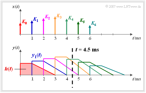
We assume an impulse response $h(t)$ which is first constant for one millisecond and then decreases linearly to zero until $t = 3 \,\text{ms}$ .

If a Dirac impulse $K_0 \cdot \delta(t)$ is applied to the input of this low-pass filter, the output signal $y(t)$ has the same shape as the impulse response $h(t)$.
The situation is shown in red in the figure.
A $T= 1 \,\text{ms}$ shifted Dirac impulse with weight $K_1 > K_0$ results in the output signal $y_1(t)$ which is delayed with respect to the red signal and increased in amplitude.

An interpretation of "Convolution"

Now we consider the input signal consisting of seven differently weighted and shifted Dirac impulses

$$x( t ) = \sum\limits_{n = 0}^6 {K_n \cdot \delta ( {t - n \cdot T} ),}$$

which can be understood as a time–discrete approximation of a time–continuous signal.

The signal at the output of the linear system is the sum of the seven partial signals marked with different colors in the figure:

$$y( t ) = \sum\limits_{n = 0}^6 {K_n \cdot h( {t - n \cdot T} ).}$$

We now look at the signal value at time $t = 4.5T$ (see dotted lines):

$$y( {t = 4.5T} ) = K_2 \cdot h( {2.5T} ) + K_3 \cdot h(1.5 T ) + K_4 \cdot h( 0.5 T ).$$

The output signal value is thus only determined by the input signal values $K_2$, $K_3$ and $K_4$. The influence of

$K_4$ due to $h(0.5T) = 1$ is the greatest,
$K_3$ due to $h(1.5T) = 0.75$ is less strong, and
$K_2$ due to $h(2.5T) = 0.25$ is the lowest.

Proof of the Convolution Theorem

$\text{Definition: }$ The following relation of time functions is called $x_1(t)$ and $x_2(t)$ the $\text{convolution}$ and represents this functional relation with a star:

$$x_{\rm{1} } (t) * x_{\rm{2} } (t) = \int_{ - \infty }^{ + \infty } {x_1 ( \tau ) } \cdot x_2 ( {t - \tau } ) \hspace{0.1cm}{\rm d}\tau.$$

This results in the following $\text{Fourier correspondence}$:

$$X_1 ( f ) \cdot X_2 ( f )\hspace{0.1cm}\bullet\!\!\!-\!\!\!-\!\!\!-\!\!\circ\hspace{0.1cm}{ {x} }_{\rm{1} } ( t ) * { {x} }_{\rm{2} } (t ).$$

$\text{Proof: }$ The Fourier integrals of functions $x_1(t)$ and $x_2(t)$ are with modified integration variables:

$$X_1 ( f ) = \int_{ - \infty }^{ + \infty } {x_1 ( \tau )} \cdot {\rm{e} }^{ - {\rm{j} }2{\rm{\pi } }f\tau }\hspace{0.1cm} {\rm{d } }\tau{\rm{,} }$$

$$X_2 ( f ) = \int_{ - \infty }^{ + \infty } {x_2 ( {t\hspace{0.05cm}'} ) } \cdot {\rm{e} }^{ - {\rm{j} }2{\rm{\pi } }ft\hspace{0.05cm}'}\hspace{0.1cm} {\rm{d} }t\hspace{0.05cm}'{\rm{.} }$$

If you form the product of the spectral functions, you get

$$X_1 (f) \cdot X_2 (f) = \int_{ - \infty }^{ + \infty } {\int_{ - \infty }^{ + \infty } {x_1 ( \tau ) \hspace{0.05 cm}\cdot } }\hspace{0.05 cm} x_2 ( {t\hspace{0.05cm}'} ) \cdot {\rm{e} }^{ - {\rm{j} }2{\rm{\pi } }f\left( {\tau + t\hspace{0.05cm}'} \right) }\hspace{0.1cm} {\rm d} \tau \hspace{0.1cm}{\rm d}t\hspace{0.05cm}'{\rm{.} }$$

With the substitution $t = \tau + t\hspace{0.05cm}'$ results:

$$X_1 ( f ) \cdot X_2 ( f ) = \int_{ - \infty }^{ + \infty } {\left[ {\int_{ - \infty }^{ + \infty } {x_1 ( \tau )} \cdot x_2 ( {t - \tau} )\hspace{0.1cm}{\rm{d } } }\tau \right] } \cdot {\rm{e} }^{ - {\rm{j} }2{\rm{\pi } }ft}\hspace{0.1cm} {\rm{d} }t{\rm{.} }$$

This equation already takes into account that the exponential function is independent of the inner integration variable ⇒ $τ$ acts only as factor of the inner integral.

If we now denote the product of the two spectra with $P(f)$ and the corresponding time function with $p(t)$, the corresponding Fourier integral is

$$P(f) = X_1 ( f ) \cdot X_2 ( f ) =\int_{ - \infty }^{ + \infty } {p( t )} \cdot {\rm{e} }^{ - {\rm{j} }2{\rm{\pi } }ft} \hspace{0.1cm}{\rm{d} }t{\rm{.} }$$