Exercise 3.2: Expected Value Calculations

Two-dimensional
probability mass function

We consider the following probability mass functions $\rm (PMF)$:

$$P_X(X) = \big[1/2,\ 1/8,\ 0,\ 3/8 \big],$$

$$P_Y(Y) = \big[1/2,\ 1/4,\ 1/4,\ 0 \big],$$

$$P_U(U) = \big[1/2,\ 1/2 \big],$$

$$P_V(V) = \big[3/4,\ 1/4\big].$$

For the associated random variables, let:

$X= \{0,\ 1,\ 2,\ 3\}$, $Y= \{0,\ 1,\ 2,\ 3\}$, $U = \{0,\ 1\}$, $V = \{0, 1\}$.

Often, for such discrete random variables, one must have to calculate different expected values of the form

$${\rm E} \big [ F(X)\big ] =\hspace{-0.3cm} \sum_{x \hspace{0.05cm}\in \hspace{0.05cm}\hspace{-0.03cm} {\rm supp} (P_X)} \hspace{-0.1cm} P_{X}(x) \cdot F(x). $$

Here, denote:

$P_X(X)$ denotes the probability mass function of the discrete random variable $X$.
The "support" of $P_X$ includes all those realisations $x$ of the random variable $X$ with non-vanishing probability.
Formally, this can be written as

$${\rm supp} (P_X) = \{ x: \hspace{0.25cm}x \in X \hspace{0.15cm}\underline{\rm and} \hspace{0.15cm} P_X(x) \ne 0 \} \hspace{0.05cm}.$$

$F(X)$ is an (arbitrary) real-valued function that can be specified in the entire domain of definition of the random variable $X$ .

In the task, the expected values for various functions $F(X)$ are to be calculated, among others for

$F(X)= 1/P_X(X)$,
$F(X)= P_X(X)$,
$F(X)= - \log_2 \ P_X(X)$.

Hints:

The exercise belongs to the chapter Some preliminary remarks on two-dimensional random variables.
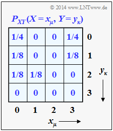
The two one-dimensional probability mass functions $P_X(X)$ and $P_Y(Y)$ result from the presented 2D–PMF $P_{XY}(X,\ Y)$, as will be shown in Exercise 3.2Z.
The binary probability mass functions $P_U(U)$ and $P_V(V)$ are obtained according to the modulo operations $U = X \hspace{0.1cm}\text{mod} \hspace{0.1cm}2$ and $V = Y \hspace{0.1cm}\text{mod} \hspace{0.1cm} 2$.

Questions

${\rm E}\big[1/P_X(X)\big] \ = \ $

${\rm E}\big[1/P_{\hspace{0.04cm}Y}(\hspace{0.02cm}Y\hspace{0.02cm})\big] \ = \ $

${\rm E}\big[P_X(X)\big] \ = \ $

${\rm E}\big[P_Y(Y)\big] \ = \ $

${\rm E}\big[P_Y(X)\big] \ = \ $

${\rm E}\big[P_X(Y)\big] \ = \ $

	${\rm E}\big[- \log_2 \ P_U(U)\big]$ gives the entropy of the random variable $U$.
	${\rm E}\big[- \log_2 \ P_V(V)\big]$ gives the entropy of the random variable $V$.
	${\rm E}\big[- \log_2 \ P_V(U)\big]$ gives the entropy of the random variable $V$.

Solution

(1) In general, the following applies to the expected value of the function $F(X)$ with respect to the random variable $X$:

$${\rm E} \left [ F(X)\right ] = \hspace{-0.4cm} \sum_{x \hspace{0.05cm}\in \hspace{0.05cm} {\rm supp} (P_X)} \hspace{-0.2cm} P_{X}(x) \cdot F(x) \hspace{0.05cm}.$$

In the present example, $X = \{0,\ 1,\ 2,\ 3\}$ and $P_X(X) = \big [1/2, \ 1/8, \ 0, \ 3/8\big ]$.

Because of $P_X(X = 2) = 0$ , the quantity to be taken into account (the "support") in the above summation thus results in

$${\rm supp} (P_X) = \{ 0\hspace{0.05cm}, 1\hspace{0.05cm}, 3 \} \hspace{0.05cm}.$$

With $F(X) = 1/P_X(X)$ one further obtains:

$${\rm E} \big [ 1/P_X(X)\big ] = \hspace{-0.4cm} \sum_{x \hspace{0.05cm}\in \hspace{0.05cm} \{ 0\hspace{0.05cm},\hspace{0.05cm} 1\hspace{0.05cm},\hspace{0.05cm} 3 \}} \hspace{-0.4cm} P_{X}(x) \cdot {1}/{P_X(x)} = \hspace{-0.4cm} \sum_{x \hspace{0.05cm}\in \hspace{0.05cm} \{ 0\hspace{0.05cm},\hspace{0.05cm} 1\hspace{0.05cm},\hspace{0.05cm} 3 \}} \hspace{-0.3cm} 1 \hspace{0.15cm}\underline{ = 3} \hspace{0.05cm}.$$

The second expected value gives the same result with ${\rm supp} (P_Y) = \{ 0\hspace{0.05cm}, 1\hspace{0.05cm}, 2 \} $ :

$${\rm E} \left [ 1/P_Y(Y)\right ] \hspace{0.15cm}\underline{ = 3}.$$

(2) In both cases, the index of the probability mass function is identical with the random variable $(X$ or $Y)$ and we obtain

$${\rm E} \big [ P_X(X)\big ] = \hspace{-0.3cm} \sum_{x \hspace{0.05cm}\in \hspace{0.05cm} \{ 0\hspace{0.05cm},\hspace{0.05cm} 1\hspace{0.05cm},\hspace{0.05cm} 3 \}} \hspace{-0.3cm} P_{X}(x) \cdot {P_X(x)} = (1/2)^2 + (1/8)^2 + (3/8)^2 = 13/32 \hspace{0.15cm}\underline{ \approx 0.406} \hspace{0.05cm},$$

$${\rm E} \big [ P_Y(Y)\big ] = \hspace{-0.3cm} \sum_{y \hspace{0.05cm}\in \hspace{0.05cm} \{ 0\hspace{0.05cm},\hspace{0.05cm} 1\hspace{0.05cm},\hspace{0.05cm} 2 \}} \hspace{-0.3cm} P_Y(y) \cdot P_Y(y) = (1/2)^2 + (1/4)^2 + (1/4)^2 \hspace{0.15cm}\underline{ = 0.375} \hspace{0.05cm}.$$

(3) The following equations apply here:

$${\rm E} \big [ P_Y(X)\big ] = \hspace{-0.3cm} \sum_{x \hspace{0.05cm}\in \hspace{0.05cm} \{ 0\hspace{0.05cm},\hspace{0.05cm} 1\hspace{0.05cm},\hspace{0.05cm} 3 \}} \hspace{-0.3cm} P_{X}(x) \cdot {P_Y(x)} = \frac{1}{2} \cdot \frac{1}{2} + \frac{1}{8} \cdot \frac{1}{4} + \frac{3}{8} \cdot 0 = 9/32 \hspace{0.15cm}\underline{ \approx 0.281} \hspace{0.05cm},$$

The expected value formation here refers to $P_X(·)$, i.e. to the random variable $X$.
$P_Y(·)$ is the formal function without (direct) reference to the random variable $Y$.
The same numerical value is obtained for the second expected value (this does not have to be the case in general):

$${\rm E} \big [ P_X(Y)\big ] = \hspace{-0.3cm} \sum_{y \hspace{0.05cm}\in \hspace{0.05cm} \{ 0\hspace{0.05cm},\hspace{0.05cm} 1\hspace{0.05cm},\hspace{0.05cm} 2 \}} \hspace{-0.3cm} P_{Y}(y) \cdot {P_X(y)} = \frac{1}{2} \cdot \frac{1}{2} + \frac{1}{4} \cdot \frac{1}{8} + \frac{1}{4} \cdot 0 = 9/32 \hspace{0.15cm}\underline{ \approx 0.281} \hspace{0.05cm}.$$

(4) We first calculate the three expected values:

$${\rm E} \big [-{\rm log}_2 \hspace{0.1cm} P_U(U)\big ] = \frac{1}{2} \cdot {\rm log}_2 \hspace{0.1cm} \frac{2}{1} + \frac{1}{2} \cdot {\rm log}_2 \hspace{0.1cm} \frac{2}{1} \hspace{0.15cm}\underline{ = 1\ {\rm bit}} \hspace{0.05cm},$$

$${\rm E} \big [-{\rm log}_2 \hspace{0.1cm} P_V(V)\big ] = \frac{3}{4} \cdot {\rm log}_2 \hspace{0.1cm} \frac{4}{3} + \frac{1}{4} \cdot {\rm log}_2 \hspace{0.1cm} \frac{4}{1} \hspace{0.15cm}\underline{ = 0.811\ {\rm bit}} \hspace{0.05cm},$$

$${\rm E} \big [-{\rm log}_2 \hspace{0.1cm} P_V(U)\big ] = \frac{1}{2} \cdot {\rm log}_2 \hspace{0.1cm} \frac{4}{3} + \frac{1}{2} \cdot {\rm log}_2 \hspace{0.1cm} \frac{4}{1} \hspace{0.15cm}\underline{ = 1.208\ {\rm bit}} \hspace{0.05cm}.$$

Accordingly, the first two statements are correct:

The entropy $H(U) = 1$ bit can be calculated according to the first equation. It applies to the binary random variable $U$ with equal probabilities.
The entropy $H(V) = 0.811$ bit is calculated according to the second equation. Due to the probabilities $3/4$ and $1/4$ , the entropy (uncertainty) is smaller here than for the random variable $U$.
The third expected value cannot indicate the entropy of a binary random variable, which is always limited to $1$ (bit) , simply because of the result $(1.208$ bit$)$ .