Basics of Convolutional Coding

# OVERVIEW OF THE THIRD MAIN CHAPTER #

This third main chapter discusses convolutional codes, first described in 1955 by $\text{Peter Elias}$ [Eli55]^[1].

While for linear block codes $($see $\text{first main chapter}$$)$ and Reed-Solomon codes $($see "second main chapter"$)$ the code word length is $n$ in each case,

the theory of convolutional codes is based on "semi-infinite" information and code sequences. Similarly, "maximum likelihood decoding" using the $\text{Viterbi algorithm}$ per se yields the entire sequence.

Specifically, this chapter discusses:

Important definitions for convolutional codes: »code rate«, »memory«, » influence length«, » free distance«,
»similarities« and »differences« to linear block codes,
»generator matrix« and »transfer function matrix« of a convolutional code,
»fractional-rational transfer functions« for systematic convolutional codes,
description with »state transition diagram« and »trellis diagram«,
»termination« and »puncturing« of convolutional codes,
»decoding« of convolutional codes ⇒ »Viterbi algorithm«,
»weight enumerator functions« and approximations for the »bit error probability«.

Alternativ:

Important definitions for convolutional codes: $\text{code rate}$, $\text{memory}$, $\text{influence length}$, $\text{free distance}$;
$\text{similarities}$ and $\text{differences}$ to linear block codes;
»generator matrix« and »transfer function matrix« of a convolutional code,
»fractional-rational transfer functions« for systematic convolutional codes,
description with »state transition diagram« and »trellis diagram«,
»termination« and »puncturing« of convolutional codes,
»decoding« of convolutional codes ⇒ »Viterbi algorithm«,
»weight enumerator functions« and approximations for the »bit error probability«.

Requirements and definitions

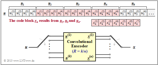
We consider in this chapter an infinite binary information sequence $\underline{u}$ and divide it into information blocks $\underline{u}_i$ of $k$ bits each. One can formalize this fact as follows:

\[\underline{\it u} = \left ( \underline{\it u}_1, \underline{\it u}_2, \hspace{0.05cm} \text{...} \hspace{0.05cm}, \underline{\it u}_i , \hspace{0.05cm} \text{...} \hspace{0.05cm}\right ) \hspace{0.3cm}{\rm with}\hspace{0.3cm} \underline{\it u}_i = \left ( u_i^{(1)}, u_i^{(2)}, \hspace{0.05cm} \text{...} \hspace{0.05cm}, u_i^{(k)}\right )\hspace{0.05cm},\]

\[u_i^{(j)}\in {\rm GF(2)}\hspace{0.3cm}{\rm for} \hspace{0.3cm}1 \le j \le k \hspace{0.5cm}\Rightarrow \hspace{0.5cm} \underline{\it u}_i \in {\rm GF}(2^k)\hspace{0.05cm}.\]

Such a sequence without negative indices is called semi–infinite.

$\text{Definition:}$ In a binary convolutional code, a code word $\underline{x}_i$ consisting of $n$ code bit is output at time $i$:

\[\underline{\it x}_i = \left ( x_i^{(1)}, x_i^{(2)}, \hspace{0.05cm} \text{...} \hspace{0.05cm}, x_i^{(n)}\right )\in {\rm GF}(2^n)\hspace{0.05cm}.\]

This results according to

the $k$ bit of the current information block $\underline{u}_i$, and

the $m$ previous information blocks $\underline{u}_{i-1}$, ... , $\underline{u}_{i-m}$.

Dependencies for a convolutional encoder with $m = 2$ Korrektur

The diagram opposite illustrates this fact for the parameters

$$k = 4, \ n = 7, \ m = 2,\ i = 4.$$

The $n = 7$ code bits $x_4^{(1)}$, ... , $x_4^{(7)}$ generated at time $i = 4$ may depend $($directly$)$ on the $k \cdot (m+1) = 12$ information bits marked in red and are generated by modulo-2 additions.

Drawn in yellow is a $(n, k)$ convolutional encoder. Note that the vector $\underline{u}_i$ and the sequence $\underline{u}^{(i)}$ are fundamentally different:

While $\underline{u}_i = (u_i^{(1)}, u_i^{(2)}$, ... , $u_i^{(k)})$ summarizes $k$ parallel information bits at time $i$,

$\underline{u}^i = (u_1^{(i)}$, $u_2^{(i)}, \ \text{...})$ denotes the $($horizontal$)$ sequence at $i$–th input of the convolutional encoder.

$\text{Some definitions related to convolutional codes:}$

The code rate results as for the block codes to $R = k/n$.

Perceive $m$ as the memory of the code and the "convolutional code" itself with ${\rm CC} \ (n, k, m)$.

This gives the constraint length $\nu = m + 1$ of the convolutional code.

For $k > 1$ one often gives these parameters also in bits: $m_{\rm bit} = m \cdot k$ resp. $\nu_{\rm bit} = (m + 1) \cdot k$.

Similarities and differences compared to block codes

From the $\text{definition}$ on the previous page, it is evident that a binary convolutional code with $m = 0$ $($i.e., without memory$)$ would be identical to a binary block code as described in the first main chapter. We exclude this limiting case and therefore assume always for the following:

The memory $m$ be greater than or equal to $1$.

The influence length $\nu$ be greater than or equal to $2$.

$\text{Example 1:}$ For a $(7, 4)$ block code, the code word $\underline {x}_4$ depends only on the information word $\underline{u}_4$ but not on $\underline{u}_2$ and $\underline{u}_3$, as in the "example convolutional codes" $($with $m = 2)$ on the last page.

Dependencies on a $(7, 4)$ block code at time $i = 4$

For example, if

$$x_4^{(1)} = u_4^{(1)}, \ x_4^{(2)} = u_4^{(2)},$$

$$x_4^{(3)} = u_4^{(3)}, \ x_4^{(4)} = u_4^{(4)}$$

as well as

$$x_4^{(5)} = u_4^{(1)}+ u_4^{(2)}+u_4^{(3)}\hspace{0.05cm},$$

$$x_4^{(6)} = u_4^{(2)}+ u_4^{(3)}+u_4^{(4)}\hspace{0.05cm},$$

$$x_4^{(7)} = u_4^{(1)}+ u_4^{(2)}+u_4^{(4)}\hspace{0.05cm},$$

applies then it is a so-called "systematic Hamming code" $\text{HS (7, 4, 3)}$. In the graph, these special dependencies for $x_4^{(1)}$ and $x_4^{(7)}$ are drawn in red.

In a sense, one could also interpret a $(n, k)$ convolutional code with memory $m ≥ 1$ as a block code whose code parameters $n\hspace{0.05cm}' \gg n$ and $k\hspace{0.05cm}' \gg k$ would have to assume much larger values than those of the present convolutional code.

However, because of the large differences in description, properties, and especially decoding, we consider convolutional codes to be something completely new in this learning tutorial. The reasons for this are as follows:

A block coder converts block-by-block information words of length $k$ bits into code words of length $n$ bits each. In this case, the larger its code word length $n$, the more powerful the block code is. For a given code rate $R = k/n$ this also requires a large information word length $k$.
In contrast, the correction capability of a convolutional code is essentially determined by its memory $m$. The code parameters $k$ and $n$ are mostly chosen very small here $(1, \ 2, \ 3, \ \text{...})$. Thus, only very few and, moreover, very simple convolutional codes are of practical importance.
Even with small values for $k$ and $n$, a convolutional encoder transfers a whole sequence of information bits $(k\hspace{0.05cm}' → ∞)$ into a very long sequence of code bits $(n\hspace{0.05cm}' = k\hspace{0.05cm}'/R)$. Such a code thus often provides a large correction capability as well.
There are efficient convolutional decoders, for example the $\text{Viterbi algorithm}$ and the $\text{BCJR algorithm}$, which can process reliability information about the channel ⇒ "soft decision input" and provide reliability information about the decoding result ⇒ "soft decision output".
Please note: The terms "convolutional code" and "convolutional encoder" should not be confused:

The "convolutional code" ${\rm CC} \ (n, \ k, \ m)$ ⇒ $R = k/n$ is understood as "the set of all possible code sequences $\underline{x}$ $($at the output$)$ that can be generated with this code considering all possible information sequences $\underline{u}$ $($at the input$)$".

There are several "convolutional encoders" that realize the same "convolutional code".

Rate 1/2 convolutional encoder

Die beiden Bilder zusammen

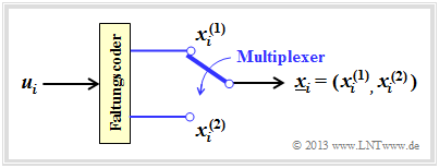
Convolutional encoder $(n = 2, \hspace{0.05cm} k = 1)$ for one bit $u_i$

Convolutional encoder $(n = 2, \hspace{0.05cm} k = 1)$ for the information sequence $\underline{u}$

The graph on the right shows a $(n = 2, \hspace{0.05cm} k = 1)$ convolutional encoder.

At clock time $i$ the information bit $u_i$ is present at the encoder input and the $2$–bit code block $\underline{x}_i = (x_i^{(1)}, \ x_i^{(2)})$ is output.

To generate two codebits $x_i^{(1)}$ and $x_i^{(2)}$ from a single information bit, the convolutional encoder must include at least one memory element:

$$k = 1\hspace{0.05cm}, \ n = 2 \hspace{0.3cm}\Rightarrow \hspace{0.3cm} m \ge 1 \hspace{0.05cm}.$$

Taking into account the $($half–infinite$)$ long information sequence $\underline{u}$ the model results according to the second graph.

$\text{Example 2:}$ The graphic shows a convolutional encoder for the parameters $k = 1, \ n = 2$ and $m = 1$.

Convolutional encoder with $k = 1, \ n = 2, \ m = 1$ and example sequences.
The square with label $D$ $($"delay"$)$ indicates a memory element.

This is a "systematic" convolutional encoder, characterized by

$$x_i^{(1)} = u_i.$$

The second output returns $x_i^{(2)} = u_i + u_{i-1}$.

In the example output sequence $\underline{x}$ after multiplexing all $x_i^{(1)}$ are labeled red and all $x_i^{(2)}$ are labeled blue.

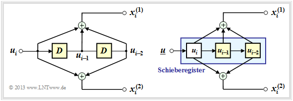
Faltungscoder $(k = 1, \ n = 2, \ m = 2)$ in zwei verschiedenen Darstellungen

$\text{Example 3:}$ The diagram shows a $(n = 2, \ k = 1)$ convolutional encoder with $m = 2$ memory elements:

On the left is shown the equivalent circuit.
On the right is a realization form of this encoder.

The two information bits are:

\[x_i^{(1)} = u_{i} + u_{i-1}+ u_{i-2} \hspace{0.05cm},\]

\[x_i^{(2)} = u_{i} + u_{i-2} \hspace{0.05cm}.\]

Because $x_i^{(1)} ≠ u_i$ this is not a systematic code.

It can be seen:

The information sequence $\underline{u}$ is stored in a shift register of length $L = m + 1 = 3$ .

At the clock time $i$ the left memory element contains the current information bit $u_i$, which is shifted one place to the right at each of the next clock times.

The number of yellow squares again gives the memory $m = 2$ of the encoder.

From the two plots it is clear that $x_i^{(1)}$ and $x_i^{(2)}$ can each be interpreted as the output of a "digital filter" over the Galois field ${\rm GF(2)}$ where both filters operate in parallel with the same input sequence $\underline{u}$ .

Since (in general terms) the output signal of a filter results from the "convolution" of the input signal with the filter impulse response, this is referred to as convolutional coding.

Convolutional encoder with two inputs

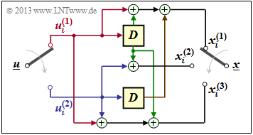
Convolutional encoder with $k = 2$ and $n = 3$

Now consider a convolutional encoder that generates code bits from $k = 2$ information bits $n = 3$ .

The information sequence $\underline{u}$ is divided into blocks of two bits each.
At the clock time $i$ bit $u_i^{(1)}$ is present at the upper input and $u_i^{(2)}$ is present at the lower input.
For the $n = 3$ code bits at time $i$ then holds:

\[x_i^{(1)} = u_{i}^{(1)} + u_{i-1}^{(1)}+ u_{i-1}^{(2)} \hspace{0.05cm},\]

\[x_i^{(2)} = u_{i}^{(2)} + u_{i-1}^{(1)} \hspace{0.05cm},\]

\[x_i^{(3)} = u_{i}^{(1)} + u_{i}^{(2)}+ u_{i-1}^{(1)} \hspace{0.05cm}.\]

In the graph, the info–bits $u_i^{(1)}$ and $u_i^{(2)}$ are marked red and blue, respectively, and the previous info–bits $u_{i-1}^{(1)}$ and $u_{i-1}^{(2)}$ are marked green and brown, respectively.

To be noted:

The memory $m$ is is equal to the maximum memory cell count in a branch ⇒ here $m = 1$.

The influence length $\nu$ is equal to the sum of all memory elements. ⇒ hier $\nu = 2$.

All memory elements are set to zero at the beginning of the coding (initialization ).

The code defined herewith is the set of all possible code sequences $\underline{x}$, which result when all possible information sequences $\underline{u}$ are entered. Both $\underline{u}$ and $\underline{x}$ are thereby (temporally) unbounded.

$\text{Example 4:}$ Let the information sequence be $\underline{u} = (0, 1, 1, 0, 0, 0, 1, 1, \ \text{ ...})$. This gives the subsequences $\underline{u}^{(1)} = (0, 1, 0, 1, \ \text{ ...})$ and $\underline{u}^{(2)} = (1, 0, 0, 1, \ \text{ ...})$.

With the specification $u_0^{(1)} = u_0^{(2)} = 0$ it follows from the above equations for the $n = 3$ code bits.

in the first coding step $(i = 1)$:

\[x_1^{(1)} = u_{1}^{(1)} = 0 \hspace{0.05cm},\hspace{0.4cm} x_1^{(2)} = u_{1}^{(2)} = 1 \hspace{0.05cm},\hspace{0.4cm} x_1^{(3)} = u_{1}^{(1)} + u_{1}^{(2)} = 0+1 = 1 \hspace{0.05cm},\]

in the second coding step $(i = 2)$:

\[x_2^{(1)} =u_{2}^{(1)} + u_{1}^{(1)}+ u_{1}^{(2)} = 1 + 0 + 1 = 0\hspace{0.05cm},\hspace{0.4cm} x_2^{(2)} = u_{2}^{(2)} + u_{1}^{(1)} = 0+0 = 0\hspace{0.05cm},\hspace{0.4cm} x_2^{(3)} = u_{2}^{(1)} + u_{2}^{(2)}+ u_{1}^{(1)} = 1 + 0+0 =1\hspace{0.05cm},\]

at the third coding step $(i = 3)$:

\[x_3^{(1)} =u_{3}^{(1)} + u_{2}^{(1)}+ u_{2}^{(2)} = 0+1+0 = 1\hspace{0.05cm},\hspace{0.4cm} x_3^{(2)} = u_{3}^{(2)} + u_{2}^{(1)} = 0+1=1\hspace{0.05cm},\hspace{0.4cm} x_3^{(3)} =u_{3}^{(1)} + u_{3}^{(2)}+ u_{2}^{(1)} = 0+0+1 =1\hspace{0.05cm},\]

and finally in the fourth coding step $(i = 4)$:

\[x_4^{(1)} = u_{4}^{(1)} + u_{3}^{(1)}+ u_{3}^{(2)} = 1+0+0 = 1\hspace{0.05cm},\hspace{0.4cm} x_4^{(2)} = u_{4}^{(2)} + u_{3}^{(1)} = 1+0=1\hspace{0.05cm},\hspace{0.4cm} x_4^{(3)}= u_{4}^{(1)} + u_{4}^{(2)}+ u_{3}^{(1)} = 1+1+0 =0\hspace{0.05cm}.\]

Thus the code sequence is after the multiplexer: $\underline{x} = (0, 1, 1, 0, 0, 1, 1, 1, 1, 1, 1, 0, \ \text{...})$.

Exercises for the chapter

Exercise 3.1: Analysis of a Convolutional Encoder

Exercise 3.1Z: Convolution Codes of Rate 1/2

References

↑ Elias, P.: Coding for Noisy Channels. In: IRE Conv. Rec. Part 4,pp. 37-47, 1955.

[Eli55-1] Elias, P.: Coding for Noisy Channels. In: IRE Conv. Rec. Part 4,pp. 37-47, 1955.

[1]