Exercise 4.10: Union Bound

Signal space constellations with $N=2$ and $M=3$

The so-called "Union Bound" gives an upper bound for the error probability of a non-binary transmission system $(M > 2)$.

The actual (average) error probability is generally given as follows:

$${\rm Pr}({ \cal E}) \hspace{-0.1cm} \ = \ \hspace{-0.1cm} \sum\limits_{i = 0 }^{M-1} {\rm Pr}(m_i) \cdot {\rm Pr}({ \cal E}\hspace{0.05cm}|\hspace{0.05cm} m_i ) \hspace{0.05cm},$$

$$ {\rm Pr}({ \cal E}\hspace{0.05cm}|\hspace{0.05cm} m_i ) \hspace{-0.1cm} \ = \ \hspace{-0.1cm} {\rm Pr} \left [ \bigcup_{k \ne i} { \cal E}_{ik}\right ] \hspace{0.05cm},\hspace{0.2cm}{ \rm where}\hspace{0.2cm} { \cal E}_{ik}\text{:} \ \ \boldsymbol{ r }{\rm \hspace{0.15cm}is \hspace{0.15cm}closer \hspace{0.15cm}to \hspace{0.15cm}}\boldsymbol{ s }_k {\rm \hspace{0.15cm}than \hspace{0.15cm}to \hspace{0.15cm}the \hspace{0.15cm}setpoint \hspace{0.15cm}}\boldsymbol{ s }_i \hspace{0.05cm}.$$

The simpler Union Bound provides an upper bound on the falsification probability assuming that message $m_i$ $($or signal $\boldsymbol{s}_i)$ was sent:

$$p_{{\rm UB}\hspace{0.05cm}| \hspace{0.05cm}\boldsymbol{ s }_i} \hspace{-0.1cm} \ \ge \ \hspace{-0.1cm} {\rm Pr}({ \cal E}\hspace{0.05cm}|\hspace{0.05cm} \boldsymbol{ s }_i ) = {\rm Pr}({ \cal E}\hspace{0.05cm}|\hspace{0.05cm} m_i )\hspace{0.05cm},\ $$

$$ p_{{\rm UB}\hspace{0.05cm}| \hspace{0.05cm}\boldsymbol{ s }_i} \hspace{-0.1cm} \ = \ \hspace{-0.2cm}\sum\limits_{k = 0 ,\hspace{0.1cm} k \ne i}^{M-1}\hspace{-0.1cm} {\rm Pr}({ \cal E}_{ik}) = \hspace{-0.1cm}\sum\limits_{k = 0, \hspace{0.1cm} k \ne i}^{M-1}\hspace{-0.1cm}{\rm Q} \left ( \frac{d_{ik}/2}{\sigma_n} \right )\hspace{0.05cm}. $$

The following abbreviations are used:

${\rm Q}(x)$ is the complementary Gaussian error function;
$d_{ik}$ denotes the distance between the signal points $\boldsymbol{s}_i$ and $\boldsymbol{s}_k$;
$\sigma_n$ is the rms value (⇒ root of the variance) of the additive white Gaussian noise.

By averaging over all possible signals $\boldsymbol{s}_i$, we then arrive at the actual Union Bound :

$$p_{\rm UB} = \sum\limits_{i = 0 }^{M-1} {\rm Pr}(\boldsymbol{ s }_i) \cdot p_{{\rm UB}\hspace{0.05cm}| \hspace{0.05cm}\boldsymbol{ s }_i} \ge {\rm Pr}({ \cal E}) \hspace{0.05cm}.$$

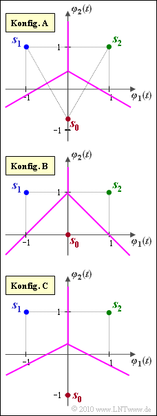
The graph shows three different signal space constellations, each with $M = 3$ signal space points $\boldsymbol{s}_0$, $\boldsymbol{s}_1$ and $\boldsymbol{s}_2$ in two-dimensional space $(N = 2)$.
The basis functions $\varphi_1(t)$ and $\varphi_2(t)$ are suitably normalized.
Thus, the signal space coordinates are also pure numerical values without unit:

$$\boldsymbol{ s }_1 = (-1, \hspace{0.1cm}+1)\hspace{0.05cm}, \hspace{0.2cm} \boldsymbol{ s }_2 = (+1, \hspace{0.1cm}+1)\hspace{0.05cm}.$$

The signal space point $\boldsymbol{s}_0$ in configuration $\rm A$ is located such that $\boldsymbol{s}_0$, $\boldsymbol{s}_1$, $\boldsymbol{s}_2$ describe an equilateral triangle. *In contrast, in configurations $\rm B$ and $\rm C$, $\boldsymbol{s}_0 = (0, 0)$ and $\boldsymbol{s}_0 = (0, \ -1)$, respectively.

Notes:

The exercise belongs to the chapter "Approximation of the Error Probability".
Use the AWGN rms value $\sigma_n = 0.5$ for all calculations.

Given the following values of the complementary Gaussian error function:

$${\rm Q}(1) \hspace{-0.1cm} \ \approx \ \hspace{-0.1cm} 0.159\hspace{0.05cm}, \hspace{0.2cm}{\rm Q}(\sqrt{2}) \approx 0.079\hspace{0.05cm}, \hspace{0.23cm}{\rm Q}(\sqrt{3}) \approx 0.042\hspace{0.05cm},$$

$${\rm Q}(2) \hspace{-0.1cm} \ \approx \ \hspace{-0.1cm} 0.023\hspace{0.05cm}, \hspace{0.2cm}{\rm Q}(2.14) \approx 0.016\hspace{0.05cm}, \hspace{0.1cm}{\rm Q}(\sqrt{5}) \approx 0.013 \hspace{0.05cm}.$$

Questions

	Configuration $\rm A$,
	Configuration $\rm B$,
	Configuration $\rm C$.

$p_{\rm UB} \ = \ $

$\ \%$

$p_{\rm UB} \ = \ $

$\ \%$

$p_{\rm UB} \ = \ $

$\ \%$

$\sigma_n \ = \ $

Solution

(1) Points $\boldsymbol{s}_1$ and $\boldsymbol{s}_2$ are the same for all configurations.

The smallest error probability occurs when $\boldsymbol{s}_0$ is farthest from $\boldsymbol{s}_1$ and $\boldsymbol{s}_2$.
This is the case for configuration C ⇒ solution 3.

(2) For configuration A, the distance between all points is the same: $d_{01} = d_{02} = d_{12} = 2$.

Therefore, to calculate the Union Bound, it is not necessary to average over all symbols, and it is valid since, for example, $\boldsymbol{s}_0$ is distorted into symbol $\boldsymbol{s}_1$ or $\boldsymbol{s}_2$ with equal probability:

$${\rm Pr}({ \cal E}) \le p_{\rm UB} = 2 \cdot {\rm Q} \left ( \frac{d_{ik}/2}{\sigma_n} \right ) = 2 \cdot {\rm Q}(2) \approx 2 \cdot 0.023 \hspace{0.1cm}\hspace{0.15cm}\underline {= 4.6\%} \hspace{0.05cm}. $$

(3) Here, the falsification probabilities differ for each symbol.

If $\boldsymbol{s}_0$ was sent, with $d_{01} = d_{02} = 2^{0.5}$ and $\sigma = 0.5$:

$$p_{{\rm UB}\hspace{0.05cm}| \hspace{0.05cm}\boldsymbol{ s }_0} = 2 \cdot {\rm Q} \left ( \frac{\sqrt{2}/2}{0.5} \right ) = 2 \cdot {\rm Q}(\sqrt{2}) = 2 \cdot 0.079 = 0.158 \hspace{0.05cm}. $$

In contrast, the other two conditional probabilities are smaller:

$$p_{{\rm UB}\hspace{0.05cm}| \hspace{0.05cm}\boldsymbol{ s }_1} = p_{{\rm UB}\hspace{0.05cm}| \hspace{0.05cm}\boldsymbol{ s }_2} \hspace{-0.1cm} \ = \ \hspace{-0.1cm} {\rm Q} \left ( \frac{{2}/2}{0.5} \right )+{\rm Q} \left ( \frac{\sqrt{2}/2}{0.5} \right )= {\rm Q}(2) +{\rm Q}(\sqrt{2}) = 0.023 + 0.079 = 0.102 \hspace{0.05cm}.$$

By averaging, we obtain for the Union Bound considering the different distances:

$$p_{\rm UB} \hspace{-0.1cm} \ = \ \hspace{-0.1cm} {1}/{3} \cdot \left [ p_{{\rm UB}\hspace{0.05cm}| \hspace{0.05cm}\boldsymbol{ s }_0} + p_{{\rm UB}\hspace{0.05cm}| \hspace{0.05cm}\boldsymbol{ s }_1} +p_{{\rm UB}\hspace{0.05cm}| \hspace{0.05cm}\boldsymbol{ s }_2}\right ]= {1}/{3} \cdot \left [ 2 \cdot {\rm Q}(\sqrt{2})+ 2 \cdot ({\rm Q}({2}) + {\rm Q}(\sqrt{2})) \right ] = {1}/{3} \cdot \left [ 4 \cdot {\rm Q}(\sqrt{2})+ 2 \cdot {\rm Q}({2}) \right ] $$

$$ \Rightarrow \hspace{0.3cm} p_{\rm UB} = {1}/{3} \cdot \left [ 4 \cdot 0.079+ 2 \cdot 0.023 \right ] \hspace{0.1cm}\hspace{0.12cm}\underline {\approx 12.1\% } \hspace{0.3cm}\Rightarrow \hspace{0.3cm} p_{\rm UB}\ge {\rm Pr}({ \cal E})\hspace{0.05cm}.$$

(4) This configuration is described by the following equations:

$$d_{01} = d_{02} = \sqrt{2^2 + 1^2}= \sqrt{5} \approx 2.24\hspace{0.2cm}, d_{12} = 2$$

$$\Rightarrow \hspace{0.3cm} p_{\rm UB} = {1}/{3} \cdot \left [ 4 \cdot {\rm Q}(\sqrt{5})+ 2 \cdot {\rm Q}({2}) \right ] = {1}/{3} \cdot \left [ 4 \cdot 0.013+ 2 \cdot 0.023 \right ]\hspace{0.1cm}\hspace{0.15cm}\underline {\approx 3.2\%} \hspace{0.05cm}. $$

(5) Let it be:

$$p_{\rm UB} = 2 \cdot {\rm Q}\left ( {1}/{\sigma_n} \right ) = 0.032 \hspace{0.3cm} \Rightarrow \hspace{0.3cm} {\rm Q}\left ( {1}/{\sigma_n} \right ) = 0.016\hspace{0.3cm} \Rightarrow \hspace{0.3cm} {1}/{\sigma_n} \approx 2.14 \hspace{0.3cm} \Rightarrow \hspace{0.3cm}\hspace{0.1cm}\hspace{0.15cm}\sigma_n \hspace{0.15cm}\underline {\approx 0.467}\hspace{0.05cm}. $$