Decoding of Linear Block Codes

Block diagram and requirements

We start from the block diagram already shown in the chapter $\text{Channel Models and Decision Structures}$ where the digital channel model used is mostly the $\text{Binary Symmetric Channel}$ $\rm (BSC)$.

For code word estimation, we use the "Maximum Likelihood Decision" $\rm (ML)$, which for binary codes ⇒ $\underline{x} \in {\rm GF}(2^n)$ at the block level gives the same result as the $\text{MAP Receiver}$.

Block diagram for decoding block codes

The task of the channel decoder can be described as follows:

The vector $\underline{v}$ after decoding (at the sink) should match the information word $\underline{u}$ as well as possible.

That is: The »block error probability« should be as small as possible:

\[{ \rm Pr(block\:error)} = { \rm Pr}( \underline{v} \ne \underline{u}) \stackrel{!}{=} { \rm minimum}\hspace{0.05cm}.\]

Because of assignments $\underline{x} = {\rm enc}(\underline{u})$ resp. $\underline{v} = {\rm enc}^{-1}(\underline{z})$ also holds:

\[{ \rm Pr(block\:error)} = { \rm Pr}( \underline{z} \ne \underline{x}) \stackrel{!}{=} { \rm minimum}\hspace{0.05cm}.\]

Sought is the most likely sent code word $\underline{y} = \underline{x} +\underline{e}$ for the given received word $\underline{x}_i$, which is passed on as result $\underline{z}$:

\[\underline{z} = {\rm arg} \max_{\underline{x}_{\hspace{0.03cm}i} \hspace{0.05cm} \in \hspace{0.05cm} \mathcal{C}} \hspace{0.1cm} {\rm Pr}( \underline{x}_{\hspace{0.03cm}i} \hspace{0.05cm}|\hspace{0.05cm} \underline{y} ) \hspace{0.05cm}.\]

For the BSC model, both $\underline{x}_i \in {\rm GF}(2^n)$ and $\underline{y} \in {\rm GF}(2^n)$, so the maximum likelihood decision rule can also be written using the $\text{Hamming distance}$ $d_{\rm H}( \underline{y}, \, \underline{x}_i)$:

\[\underline{z} = {\rm arg} \min_{\underline{x}_{\hspace{0.03cm}i} \hspace{0.05cm} \in \hspace{0.05cm} \mathcal{C}} \hspace{0.1cm} d_{\rm H}(\underline{y} \hspace{0.05cm}, \hspace{0.1cm}\underline{x}_{\hspace{0.03cm}i})\hspace{0.05cm}.\]

Principle of syndrome decoding

Assumed here is a $(n, \, k)$ block code with the parity-check matrix $\boldsymbol{\rm H}$ and the systematic code words

\[\underline{x}\hspace{0.05cm} = (x_1, x_2, \hspace{0.05cm}\text{...} \hspace{0.05cm}, x_i, \hspace{0.05cm}\text{...} \hspace{0.05cm}, x_n) = (u_1, u_2, \hspace{0.05cm}\text{...} \hspace{0.05cm}, u_k, p_1, \hspace{0.05cm}\text{...} \hspace{0.05cm}, p_{n-k})\hspace{0.05cm}. \]

With the error vector $\underline{e}$ then applies to the received word:

\[\underline{y} = \underline{x} + \underline{e} \hspace{0.05cm}, \hspace{0.4cm} \underline{y} \in \hspace{0.1cm} {\rm GF}(2^n) \hspace{0.05cm}, \hspace{0.4cm} \underline{x} \in \hspace{0.1cm} {\rm GF}(2^n) \hspace{0.05cm}, \hspace{0.4cm} \underline{e} \in \hspace{0.1cm} {\rm GF}(2^n) \hspace{0.05cm}.\]

A bit error at position $i$ ⇒ $y_i ≠ x_i$ is expressed by the »error coefficient« $e_i = 1$.

$\text{Definition:}$ The »syndrome« $\underline{s} = (s_0, s_1, \hspace{0.05cm}\text{...} \hspace{0.05cm}, s_{m-1})$ is calculated (as row resp. column vector) from the received word $\underline{y}$ and the parity-check matrix $\boldsymbol{\rm H}$ as follows:

\[\underline{s} = \underline{y} \cdot { \boldsymbol{\rm H} }^{\rm T}\hspace{0.3cm}{\rm bzw.}\hspace{0.3cm} \underline{s}^{\rm T} = { \boldsymbol{\rm H} } \cdot \underline{y}^{\rm T}\hspace{0.05cm}.\]

The vector length of $\underline{s}$ is equal to $m = n-k$ $($row number of $\boldsymbol{\rm H})$.

The syndrome $\underline{s}$ shows the following characteristics:

Because of the equation $\underline{x} \cdot { \boldsymbol{\rm H}}^{\rm T} = \underline{0}$ the syndrome $\underline{s}$ does not depend on the code word $\underline{x}$ but solely on the error vector $\underline{e}$:

\[\underline{s} = \underline{y} \cdot { \boldsymbol{\rm H}}^{\rm T} = \hspace{0.05cm} \underline{x} \cdot { \boldsymbol{\rm H}}^{\rm T} + \hspace{0.05cm} \underline{e} \cdot { \boldsymbol{\rm H}}^{\rm T} = \hspace{0.05cm} \underline{e} \cdot { \boldsymbol{\rm H}}^{\rm T} \hspace{0.05cm}.\]

For sufficiently few bit errors, $\underline{s}$ provides a clear indication of the error locations, allowing full error correction.

$\text{Example 1:}$ Starting from the systematic $\text{(7, 4, 3)}$ Hamming code, the following result is obtained for the received vector $\underline{y} = (0, 1, 1, 1, 0, 0, 1)$:

\[{ \boldsymbol{\rm H} } \cdot \underline{y}^{\rm T} = \begin{pmatrix} 1 &1 &1 &0 &1 &0 &0\\ 0 &1 &1 &1 &0 &1 &0\\ 1 &1 &0 &1 &0 &0 &1 \end{pmatrix} \cdot \begin{pmatrix} 0 \\ 1 \\ 1 \\ 1 \\ 0 \\ 0 \\ 1 \end{pmatrix} = \begin{pmatrix} 0 \\ 1 \\ 1 \end{pmatrix} = \underline{s}^{\rm T} \hspace{0.05cm}.\]

Comparing the syndrome with the $\text{parity-check equations}$ of the Hamming code, we see that

most likely the fourth symbol $(x_4 = u_4)$ of the code word has been corrupted KORREKTUR: falsified,

the code word estimator will thus yield the result $\underline{z} = (0, 1, 1, 0, 0, 0, 1)$,

the decision is correct only if only one bit was corrupted KORREKTUR: falsified during transmission.

Below are the required corrections for the $\text{(7, 4, 3)}$ Hamming code resulting from the calculated syndrome $\underline{s}$ corresponding to the columns of the parity-check matrix:

\[\underline{s} = (0, 0, 0) \hspace{0.10cm} \Rightarrow\hspace{0.10cm}{\rm no\hspace{0.15cm} correction}\hspace{0.05cm};\hspace{0.8cm}\underline{s} = (1, 0, 0)\hspace{0.10cm} \Rightarrow\hspace{0.10cm}{\rm invert}\hspace{0.15cm}p_1\hspace{0.05cm};\]

\[\underline{s} =(0, 0, 1)\hspace{0.10cm} \Rightarrow\hspace{0.10cm} {\rm invert}\hspace{0.15cm}p_3\hspace{0.05cm};\hspace{1.63cm}\underline{s} = (1, 0, 1)\hspace{0.10cm} \Rightarrow\hspace{0.10cm} {\rm invert}\hspace{0.15cm}u_1\hspace{0.05cm};\]

\[\underline{s} =(0, 1, 0)\hspace{0.10cm} \Rightarrow\hspace{0.10cm} {\rm invert}\hspace{0.15cm}p_2\hspace{0.05cm};\hspace{1.63cm}\underline{s} = (1, 1, 0)\hspace{0.10cm} \Rightarrow\hspace{0.10cm} {\rm invert}\hspace{0.15cm}u_3\hspace{0.05cm};\]

\[\underline{s} =(0, 1, 1)\hspace{0.10cm} \Rightarrow\hspace{0.10cm} {\rm invert}\hspace{0.15cm}u_4\hspace{0.05cm};\hspace{1.63cm}\underline{s} = (1, 1, 1)\hspace{0.10cm} \Rightarrow\hspace{0.10cm} {\rm invert}\hspace{0.15cm}u_2\hspace{0.05cm}. \]

Generalization of syndrome coding

We continue to assume the BSC channel model. This means:

The received vector $\underline{y}$ and the error vector $\underline{e}$ are elements of ${\rm GF}(2^n)$.

The possible code words $\underline{x}_i$ belong to the code $\mathcal{C}$, which spans a $(n-k)$-dimensional subspace of ${\rm GF}(2^n)$.

Under this assumption, we briefly summarize the results of the last sections:

Syndrome decoding is a realization possibility of maximum likelihood decoding of block codes. One decides on the code word $\underline{x}_i$ with the least Hamming distance to the received word $\underline{y}$:

\[\underline{z} = {\rm arg} \min_{\underline{x}_{\hspace{0.03cm}i} \hspace{0.05cm} \in \hspace{0.05cm} \mathcal{C}} \hspace{0.1cm} d_{\rm H}(\underline{y} \hspace{0.05cm}, \hspace{0.1cm}\underline{x}_{\hspace{0.03cm}i})\hspace{0.05cm}.\]

But the syndrome decoding is also the search for the most probable error vector $\underline{e}$ that satisfies the condition $\underline{e} \cdot { \boldsymbol{\rm H}}^{\rm T} = \underline{s}$. The "syndrome" is thereby determined by the equation

$$\underline{s} = \underline{y} \cdot { \boldsymbol{\rm H}}^{\rm T} .$$

With the $\text{Hamming weight}$ $w_{\rm H}(\underline{e})$ the second interpretation can also be mathematically formulated as follows:

\[\underline{z} = \underline{y} + {\rm arg} \min_{\underline{e}_{\hspace{0.03cm}i} \hspace{0.05cm} \in \hspace{0.05cm} {\rm GF}(2^n)} \hspace{0.1cm} w_{\rm H}(\underline{e}_{\hspace{0.03cm}i})\hspace{0.05cm}.\]

$\text{Conclusion:}$ Note that the error vector $\underline{e}$ as well as the received vector $\underline{y}$ is an element of ${\rm GF}(2^n)$ unlike the syndrome $\underline{s} \in {\rm GF}(2^m)$ with number $m = n-k$ of parity-check equations. This means, that

the association between the syndrome $\underline{s}$ and the error vector $\underline{e}$ is not unique, but

each $2^k$ error vectors lead to the same syndrome $\underline{s}$ which one groups together into a so-called "coset".

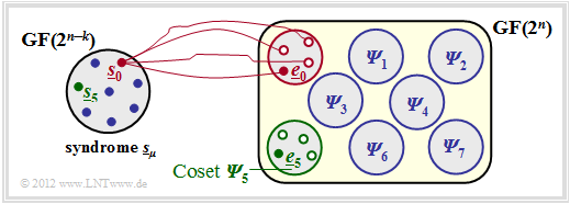
$\text{Example 2:}$ The facts shall be illustrated by the example with parameters $n = 5, \ k = 2$ ⇒ $m = n-k = 3$ .

Splitting the $2^k$ error vectors into "cosets"

You can see from this graph:

The $2^n = 32$ possible error vectors $\underline{e}$ are divided into $2^m = 8$ cosets ${\it \Psi}_0$, ... , ${\it \Psi}_7$. Explicitly drawn here are only the cosets ${\it \Psi}_0$ and ${\it \Psi}_5$.
All $2^k = 4$ error vectors of the coset ${\it \Psi}_\mu$ lead to the syndrome $\underline{s}_\mu$.
Each minor class ${\it \Psi}_\mu$ has a "leader" $\underline{e}_\mu$, namely the one with the minimum Hamming weight.

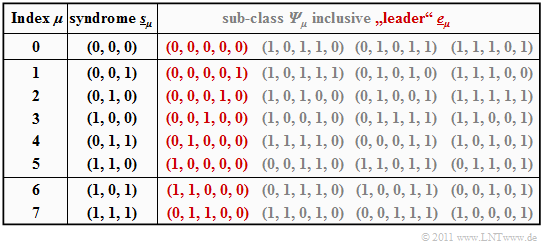
$\text{Example 3:}$ Starting from the systematic $\text{(5, 2, 3)}$ code $\mathcal{C} = \big \{ (0, 0, 0, 0, 0) \hspace{0.05cm},\hspace{0.15cm}(0, 1, 0, 1, 1) \hspace{0.05cm},\hspace{0.15cm}(1, 0, 1, 1, 0) \hspace{0.05cm},\hspace{0.15cm}(1, 1, 1, 0, 1) \big \}$ the syndrome decoding procedure is now described in detail.

Example $\text{(5, 2, 3)}$ syndrome table with cosets KORREKTUR: ""

The generator matrix and the parity-check matrix are:

\[{ \boldsymbol{\rm G} } = \begin{pmatrix} 1 &0 &1 &1 &0 \\ 0 &1 &0 &1 &1 \end{pmatrix} \hspace{0.05cm},\]

\[{ \boldsymbol{\rm H} } = \begin{pmatrix} 1 &0 &1 &0 &0 \\ 1 &1 &0 &1 &0 \\ 0 &1 &0 &0 &1 \end{pmatrix} \hspace{0.05cm}.\]

The table summarizes the final result. Note:

The index $\mu$ is not identical to the binary value of $\underline{s}_\mu$.
The order is rather given by the number of ones in the minor class leader $\underline{e}_\mu$.
For example, the syndrome $\underline{s}_5 = (1, 1, 0)$ and the syndrome $\underline{s}_6 = (1, 0, 1)$.

To derive this table, note:

The row 1 refers to the syndrome $\underline{s}_0 = (0, 0, 0)$ and the associated cosets ${\it \Psi}_0$. The most likely error sequence here is $(0, 0, 0, 0, 0)$ ⇒ no bit error, which we call the "coset leader" $\underline{e}_0$.
The other entries in the first row, namely $(1, 0, 1, 1, 0 )$, $(0, 1, 0, 1, 1)$ and $(1, 1, 1, 0, 1 )$, also each yield the syndrome $\underline{s}_0 = (0, 0, 0)$, but only result with at least three bit errors and are correspondingly unlikely.
In rows 2 to 6, the respective coset leader $\underline{e}_\mu$ contains exactly a single "$1$" $(\mu = 1$, ... , $5)$. Here $\underline{e}_\mu$ is always the most likely error pattern of the class ${\it \Psi}_\mu$. The other group members result only with at least two bit errors.
The syndrome $\underline{s}_6 = (1, 0, 1)$ is not possible with only one bit error. In creating the table, we then considered all "$5\text{ over }2 = 10$" error patterns $\underline{e}$ with weight $w_{\rm H}(\underline{e}) = 2$.
The first found sequence with syndrome $\underline{s}_6 = (1, 0, 1)$ was chosen as coset leader $\underline{e}_6 = (1, 1, 0, 0)$ . With a different probing order, the sequence $(0, 0, 1, 0, 1)$ could also have resulted from ${\it \Psi}_6$.
Similar procedure was followed in determining the leader $\underline{e}_7 = (0, 1, 1, 0, 0)$ of the cosets class ${\it \Psi}_7$ characterized by the uniform syndrome $\underline{s}_7 = (1, 1, 1)$. Also in the class ${\it \Psi}_7$ there is another sequence with Hamming weight $w_{\rm H}(\underline{e}) = 2$, namely $(1, 0, 0, 0, 1)$.

The table only needs to be created once. First, the syndrome must be determined, e.g. for the received vector $\underline{y} = (0, 1, 0, 0, 1)$:

\[\underline{s} = \underline{y} \cdot { \boldsymbol{\rm H} }^{\rm T} = \begin{pmatrix} 0 &1 &0 &0 &1 \end{pmatrix} \cdot \begin{pmatrix} 1 &1 &0 \\ 0 &1 &1 \\ 1 &0 &0 \\ 0 &1 &0 \\ 0 &0 &1 \\ \end{pmatrix} = \begin{pmatrix} 0 &1 &0 \end{pmatrix}= \underline{s}_2 \hspace{0.05cm}.\]

Using the coset leader $\underline{e}_2 = (0, 0, 0, 1, 0)$ from the above table $($red entry for $\mu =2)$ finally arrives at the decoding result:

\[\underline{z} = \underline{y} + \underline{e}_2 = (0,\hspace{0.05cm} 1,\hspace{0.05cm} 0,\hspace{0.05cm} 0,\hspace{0.05cm} 1) + (0,\hspace{0.05cm} 0,\hspace{0.05cm} 0,\hspace{0.05cm} 1,\hspace{0.05cm} 0) = (0,\hspace{0.05cm} 1,\hspace{0.05cm} 0,\hspace{0.05cm} 1,\hspace{0.05cm} 1) \hspace{0.05cm}.\]

$\text{Conclusion:}$ From these examples it is already clear that the »syndrome decoding means a considerable effort«, if one cannot use certain properties e.g. cyclic codes.

For large block code lengths, this method fails completely. Thus, to decode a $\text{BCH codes}$ $($the abbreviation stands for their inventors Bose, Chaudhuri, Hocquenghem$)$ with code parameters $n = 511$, $k = 259$ and $d_{\rm min} = 61$, one has to evaluate and store exactly $2^{511-259} \approx 10^{76}$ error patterns of length $511$.
Happily, however, there are special decoding algorithms for these and also for other codes of large block length, which lead to success with less effort

.

Coding gain - bit error rate with AWGN

We now consider the $\text{bit error rate}$ for the following constellation:

Bit error rate for the $\text{(7, 4, 3)}$ Hamming code Korrektur Gainn

Hamming code $\text{HC (7, 4, 3)}$,
AWGN–channel, characterized by the quotient $E_{\rm B}/N_0$ (in dB),
Maximum Likelihood Decoder $\rm (ML)$ with
"Hard Decision" $\rm (HD)$ and "Soft Decision" $\rm (SD)$, resp.

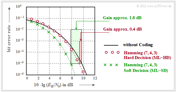
It should be noted with regard to this graph:

The black comparison curve applies e.g. to binary phase modulation $\rm (BPSK)$ without coding. For this one needs for the bit error rate $10^{-5}$ about $10 \cdot \lg \, E_{\rm B}/N_0 = 9.6 \, \rm dB$.

The red circles apply to the $\text{HC (7, 4, 3)}$ and hard decisions of the maximum likelihood decoder $\text{(ML–HD)}$. Syndrome decoding is a possible realization form for this.

This configuration brings an improvement over the comparison system only for $10 \cdot \lg \, E_{\rm B}/N_0 >6 \, \rm dB$. For $\rm BER =10^{-5}$ one only needs $10 \cdot \lg \, E_{\rm B}/N_0 \approx 9.2 \, \rm dB$.

The green crosses for $\text{HC (7, 4, 3)}$ and $\text{soft decision}$ $\text{(ML–SD)}$ are below the red curve throughout the range. For $\rm BER =10^{-5}$ this gives $10 \cdot \lg \, E_{\rm B}/N_0 \approx 7.8 \, \rm dB$.

$\text{Definition:}$ We refer as »coding gain« of a considered system configuration,

characterized by its code and
the way it is decoded,

the smaller $10 \cdot \lg \, E_{\rm B}/N_0$ required for a given bit error rate $\rm (BER)$ compared to the comparison system $($without coding$)$:

\[G_{\rm Code} (\hspace{0.05cm}\text{considered system} \hspace{0.05cm}\vert\hspace{0.05cm}{\rm BER}\hspace{0.05cm}) =10 \cdot {\rm lg}\hspace{0.1cm}{E}_{\rm B}/N_0 \hspace{0.15cm}(\hspace{0.05cm}\text{comparison system}\hspace{0.05cm}\vert\hspace{0.05cm}{\rm BER}\hspace{0.05cm})- 10 \cdot {\rm lg}\hspace{0.1cm}{E}_{\rm B}/N_0 \hspace{0.15cm}(\hspace{0.05cm}\text{considered system}\hspace{0.05cm}\vert\hspace{0.05cm}{\rm BER}\hspace{0.05cm}) \hspace{0.05cm}. \]

Applied to the above graph, one obtains:

\[G_{\rm Code} (\hspace{0.05cm}{\rm Hamming \hspace{0.1cm}(7,\hspace{0.02cm}4,\hspace{0.02cm}3), ML-HD}\hspace{0.05cm}|\hspace{0.05cm}{\rm BER} = 10^{-5}\hspace{0.05cm}) = 0.4\ {\rm dB}\hspace{0.05cm},\]

\[G_{\rm Code} (\hspace{0.05cm}{\rm Hamming \hspace{0.1cm}(7,\hspace{0.02cm}4,\hspace{0.02cm}3), ML-SD}\hspace{0.05cm}|\hspace{0.05cm}{\rm BER} = 10^{-5}\hspace{0.05cm}) = 1.8\ {\rm dB}\hspace{0.05cm}.\]

Decoding at the Binary Erasure Channel

Finally, it will be shown to what extent the decoder has to be modified

if instead of the $\text{BSC model}$ ("Binary Symmetric Channel")
the $\text{BEC model}$ ("Binary Erasure Channel") is used,

which does not produce errors but marks uncertain bits as "erasures".

$\text{Example 4:}$ We consider again as in $\text{Example 3}$ the systematic $\text{(5, 2, 3)}$ block code

$$\mathcal{C} = \big \{ (0, 0, 0, 0, 0) \hspace{0.05cm},\hspace{0.3cm}(0, 1, 0, 1, 1) \hspace{0.05cm},\hspace{0.3cm}(1, 0, 1, 1, 0) \hspace{0.05cm},\hspace{0.3cm}(1, 1, 1, 0, 1) \big \}.$$

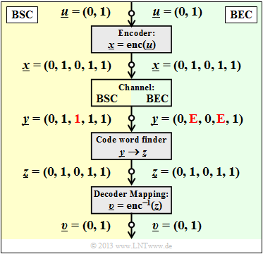
The graphic shows the system model and gives exemplary values for the individual vectors.

The left part of the picture (yellow background) is valid for "BSC" with one bit error $(0 → 1)$ at the third bit.
The right part of the picture (green background) is for "BEC" and shows two Erasures $(\rm 1 → E)$ at the second and the fourth bit.

Error correction with BSC and BEC

One recognizes:

With BSC only $t = 1$ bit error (marked in red in the left part) can be corrected due to $d_{\rm min} = 3$. If one restricts oneself to error detection, this works up to $e= d_{\rm min} -1 = 2$ bit errors.

For BEC, error detection makes no sense, because already the channel locates an uncertain bit as an "erasure" $\rm E$. The zeros and ones in the BEC received word $\underline{y}$ are safe. Therefore the error correction works here up to $e = 2$ erasures (marked in red in the right part) with certainty.

Also $e = 3$ erasures are sometimes still correctable. So $\underline{y} \rm = (E, E, E, 1, 1)$ to $\underline{z} \rm = (0, 1, 0, 1, 1)$ to be corrected since no second code word ends with two ones. But $\underline{y} \rm = (0, E, 0, E, E)$ is not correctable because of the all zero word allowed in the code.

If it is ensured that there are no more than two erasures in any received word, the BEC block error probability ${\rm Pr}(\underline{z} \ne \underline{x}) = {\rm Pr}(\underline{v} \ne \underline{u}) \equiv 0$. In contrast, the corresponding block error probability in the BSC model always has a value greater than $0$.

Since after the BEC each received word is either decoded correctly or not at all, we call here the block $\underline{y} → \underline{z}$ in the future "code word finder". An "estimation" takes place only in the BSC model.

But how does the decoding of a received word $\underline{y}$ with erasures work algorithmically?

$\text{Example 5:}$ Starting from the received word $\underline{y} \rm = (0, E, 0, E, 1)$ in $\text{Example 4}$ we formally set the output of the code word finder to $\underline{z} \rm = (0, z_2, 0, z_4, 1)$, where the symbols $z_2 \in \{0, \, 1\}$ and $z_4 \in \{0, \, 1\}$ are to be determined according to the following equation:

\[\underline{z} \cdot { \boldsymbol{\rm H} }^{\rm T}= \underline{0} \hspace{0.3cm} \Rightarrow \hspace{0.3cm} { \boldsymbol{\rm H} } \cdot \underline{z}^{\rm T}= \underline{0}^{\rm T} \hspace{0.05cm}.\]

The task is now to implement this determination equation as efficiently as possible. The following calculation steps result:

With the parity-check matrix $\boldsymbol{\rm H}$ of the $\text{(5, 2, 3)}$ block code and the vector $\underline{z} \rm = (0, z_2, 0, z_4, 1)$ is the above determination equation:

\[{ \boldsymbol{\rm H} } \cdot \underline{z}^{\rm T} = \begin{pmatrix} 1 &0 &1 &0 &0\\ 1 &1 &0 &1 &0\\ 0 &1 &0 &0 &1 \end{pmatrix} \cdot \begin{pmatrix} 0 \\ z_2 \\ 0 \\ z_4 \\ 1 \end{pmatrix} = \begin{pmatrix} 0 \\ 0 \\ 0 \end{pmatrix} \hspace{0.05cm}.\]

We sum up the "correct bits" (German: "korrekt" ⇒ subscript "K") to the vector $\underline{z}_{\rm K}$ and the "erased bits" to the vector $\underline{z}_{\rm E}$. Then we split the parity-check matrix $\boldsymbol{\rm H}$ into the corresponding submatrices $\boldsymbol{\rm H}_{\rm K}$ and $\boldsymbol{\rm H}_{\rm E}$:

\[\underline{z}_{\rm K} =(0, 0, 1)\hspace{0.05cm},\hspace{0.3cm} { \boldsymbol{\rm H} }_{\rm K}= \begin{pmatrix} 1 &1 &0\\ 1 &0 &0\\ 0 &0 &1 \end{pmatrix} \hspace{0.3cm}\Rightarrow\hspace{0.3cm} \text{Rows 1, 3 and 5 of the parity-check matrix} \hspace{0.05cm},\]

\[\underline{z}_{\rm E} = (z_2, z_4)\hspace{0.05cm},\hspace{0.35cm} { \boldsymbol{\rm H} }_{\rm E}= \begin{pmatrix} 0 &0\\ 1 &1\\ 1 &0 \end{pmatrix} \hspace{1.05cm}\Rightarrow\hspace{0.3cm} \text{Rows 2 and 4 of the parity-check matrix} \hspace{0.05cm}.\]

Remembering that in $\rm GF(2)$ subtraction equals addition, the above equation can be represented as follows:

\[{ \boldsymbol{\rm H} }_{\rm K} \cdot \underline{z}_{\rm K}^{\rm T} + { \boldsymbol{\rm H} }_{\rm E} \cdot \underline{z}_{\rm E}^{\rm T}= \underline{0}^{\rm T} \hspace{0.3cm} \Rightarrow \hspace{0.3cm} { \boldsymbol{\rm H} }_{\rm E} \cdot \underline{z}_{\rm E}^{\rm T}= { \boldsymbol{\rm H} }_{\rm K} \cdot \underline{z}_{\rm K}^{\rm T} \hspace{0.3cm} \Rightarrow \hspace{0.3cm} \begin{pmatrix} 0 &0\\ 1 &1\\ 1 &0 \end{pmatrix} \cdot \begin{pmatrix} z_2 \\ z_4 \end{pmatrix} = \begin{pmatrix} 1 &1 &0\\ 1 &0 &0\\ 0 &0 &1 \end{pmatrix} \cdot \begin{pmatrix} 0 \\ 0 \\ 1 \end{pmatrix} = \begin{pmatrix} 0 \\ 0 \\ 1 \end{pmatrix} \hspace{0.05cm}.\]

This leads to a linear system of equations with two equations for the unknown $z_2$ and $z_4$ $($each $0$ or $1)$.

From the last row follows $z_2 = 1$ and from the second row $z_2 + z_4 = 0$ ⇒ $z_4 = 1$. This gives the allowed code word $\underline{z} \rm = (0, 1, 0, 1, 1)$.