Generation of Discrete Random Variables

Pseudo-random variables

One way to generate a binary random sequence $〈z_{\rm ν}〉 ∈ \{0, 1\}$ with good statistical properties is offered by the so-called »pseudo-random generators«, also known as »PN generators«, where "PN" stands for "pseudo-noise".

These have the following properties:

The binary sequence generated by such a generator is not stochastic in a strict sense, but exhibits periodic and thus deterministic properties.
If the period length $P$ is sufficiently large, the sequence appears to an observer as random with sufficiently good statistical properties for many applications.
The advantage of a pseudo-random generator over a "real" stochastic source is that the random sequence is reproducible if a few parameters are known.

$\text{Example 1:}$ The latter property also gives rise to the main applications of pseudo-noise generators:

first, the "error frequency measurement" in digital signal transmission,
secondly, for band spreading in CDMA ("Code Division Multiple Access").

In such a "Spread Spectrum System" the transmitted signal is modulated with a binary random sequence, whose symbol repetition frequency is significantly higher than the bit frequency. This offers the possibility of multiple channel utilization. Since the same sequence must be added in phase at the receiver, the use of reproducible PN sequences is also common here.

Detailed information on bandspreading methods can be found in the chapter "UMTS - Universal Mobile Telecommunications System" of the book "Examples of Communication Systems".

Realization of PN generators

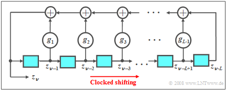
Pseudo-random generators are usually realized by feedback shift registers, where at each clock instant the content of the register is shifted one place to the right (see diagram). For the currently generated symbol, with $g_l ∈ \{0, 1\}$ and $l = 1$, ... , $L-1$:

$$z_\nu = (g_1\cdot z_{\nu-1}+g_2\cdot z_{\nu-2}+\hspace{0.1cm}\text{...}\hspace{0.1cm}+g_l\cdot z_{\nu-l}+\hspace{0.1cm}\text{...}\hspace{0.1cm}+g_{L-1}\cdot z_{\nu-L+1}+ z_{\nu-L})\hspace{0.1cm} \rm mod \hspace{0.2cm}2.$$

The binary values $z_{ν-1}$ to $z_{ν-L}$ generated at previous time points are stored in the memory cells of the shift register.
The coefficients $g_1$, ... , $g_{L-1}$ are also binary values, where a "one" indicates a feedback at the corresponding location and a "zero" indicates no feedback.
Modulo-2 addition can be implemented, for example, using an XOR operation:

Pseudo-noise generator

$$(x + y)\hspace{0.15cm} \rm mod\hspace{0.15cm}2 = \it x\hspace{0.15cm}\rm XOR\hspace{0.15cm} \it y = \left\{\begin{array}{*{2}{c}} \rm 0 & \rm if\hspace{0.15cm} \it x= y,\\ 1 & \rm if\hspace{0.15cm} \it x\neq y. \\ \end{array} \right.$$

The statistical properties of the generated pseudo-noise random sequence $〈z_{\rm ν}〉$ are essentially determined by

the »degree« $L$, and
the »feedback coefficients« $g_{\hspace{0.05cm}l}$ $($with $l = 1$, ... , $L-1)$.

A prerequisite for the generation of a PN sequence is that not all memory elements are preallocated with zeros, otherwise the modulo-2 addition would always generate the symbol "$0$".

To identify different PN generators one uses in the literature alternatively:

The »generator polynomials« of the type

$$G(D) = g_L\cdot D^L+g_{L-1}\cdot D^{L-1}+ \ \text{...} \ +g_1\cdot D+g_0 .$$

Here, $g_0 = g_L = 1$ is always to be set; $D$ is a formal parameter indicating a delay by one clock $(D^L$ indicates a delay by $L$ clocks$)$.

The »octal representation« of the binary number $(g_L\ \text{ ...} \ g_2 \ g_1 \ g_0)$. It is important that here the feedback coefficients – starting from the right with $g_0$ – are combined into triples and these are written octal $(0 \ \text{...}\ 7)$.

$\text{Example 2:}$ The generator polynomial $D^4 + D^3 + 1$ belongs to a shift register of degree $L = 4$ with the following octal representation.

$$(g_4 \ g_3 \ g_2 \ g_1 \ g_0) = (11001)_{\rm bin} = (31)_{\rm oct}. $$

Sequences of maximum length (M-sequences)

If not all $L$ memory cells of the shift register are preallocated with zeros, a periodic random sequence $〈z_ν\rangle$ always results:

Composition of some favorable generator polynomials Korrektur: identisch, Polynom

The period length $P$ of this sequence depends to a strong degree on the feedback coefficients.
For each degree $L$ there is at least one configuration with »maximum period length«

$$P_{\rm max} = \rm 2^{\it L}-\rm 1.$$

Such a PN sequence is also often referred to as »M-sequence«, where the "M" stands for "Maximum".

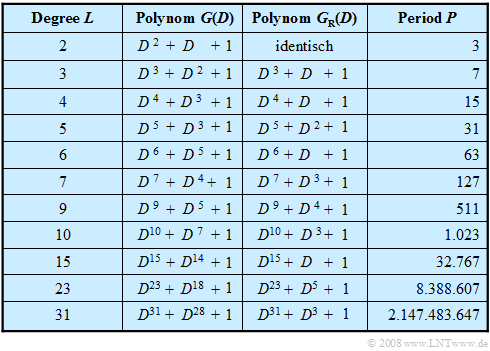
The table on the right lists PN generators of maximum length up to degree $L = 31$ .

The selection is limited to configurations with only one tap – that is, with two returns.
This means that the associated polynomials consist of only three summands.
For applications that require high speed, such generators are very useful.

$\text{For now, without proof:}$

A »M-sequence« can be recognized by the fact that the generator polynomial $G(D)$ is primitive.
As detailed in the book "Channel Coding", a polynomial $G(D)$ of degree $L$ is called »primitive« if the following condition is satisfied:

$$\frac{D^n+ 1}{G(D)} \neq 0\hspace{0.5cm} {\rm for}\hspace{0.5cm}\it n<P_{\rm max} \rm = \rm 2^{\it L}-\rm 1.$$

$\text{Example 3:}$ A shift register of degree $L = 4$ with octal identifier $(31)$ and generator polynomial $G(D) = D^4 + D^3 + 1$ leads to a sequence of maximum length:

$$P_{\rm max} = 2^4 - 1 = 15.$$

The mathematical proof for this is complex:

Using the above polynomial division for $n = 1$, ... , $14$ one must show that the quotient is always nonzero.
First the division $(D^{15} + 1)/G(D)$ may give a result without remainder.
Here it is to be considered that in the modulo-2 algebra $+1$ and $-1$ are identical.

Reciprocal polynomials

$\text{Definition:}$ The »reciprocal polynomial« associated with the generator polynomial $G(D)$ is:

$$G_{\rm R}(D)=D^{L}\cdot G(D^{-1}).$$

Between the two shift registers with polynomials $G(D)$ and $G_{\rm R}(D)$ respectively, there are the following relations:

If $G(D)$ provides a sequence of maximum length ⇒ $P_{\rm max} = 2^L - 1$, then the period length of the reciprocal polynomial $G_{\rm R}(D)$ is also maximum.
The output sequences of reciprocal configurations are inverses of each other. That is:
The sequence of $G(D)$ – read from right to left – gives the sequence of the reciprocal configuration $G_{\rm R}(D)$.

In the $\text{table above}$ the reciprocal polynomials $G_{\rm R}(D)$ associated to $G(D)$ are given in the third column up to register degree $L = 31$ .

$\text{Example 4:}$ We consider again the degree $L = 4$.

Based on the shift register structure $(31)_{\rm oct}$ we obtain for the reciprocal polynomial:

$$G_{\rm R}(D) = D^{\rm 4}\cdot (1+D^{-3} + D^{ -4})=D^{ 4}+D^{1}+\rm 1$$

and thus the configuration with the octal identifier $(23)$.

The corresponding output sequences each have the maximum period length $P_{\rm max} = 15$ and are inverses of each other:

... $0 \ 0 \ 0 \ 1 \ 0 \ 0 \ 1 \ 1 \ 0 \ 1 \ 0 \ 1 \ 1 \ 1 \ 1$ ...
... $0 \ 1 \ 0 \ 1 \ 1 \ 0 \ 0 \ 1 \ 0 \ 0 \ 0 \ 1 \ 1 \ 1 \ 1$ ...

This means that the upper initial sequence of $(31)$, read from right to left, yields the sequence of reciprocal order $(23)$ given below.
However, a cyclic phase shift of four binary digits can be seen.

The topic of this chapter is illustrated with examples in the (German language) learning video:
"Erläuterung der PN-Generatoren an einem Beispiel" $\Rightarrow$ Explanation of PN generators using an example.

==Generation of multilevel random variables==KORREKTUR: multi-level
Many high-level programming languages provide pseudo-random generators that return real random numbers $x$ equally distributed between $0$ and $1$. For example, a corresponding C function call is:

$$x = \text{random()}.$$

By successively calling this "random function", a periodically repeating sequence of real numbers is created, where all values $0 \le x < 1$ are equally likely ⇒ see chapter "Uniformly Distributed Random Variables".

However, since the period $P$ is very large, this sequence can be considered as "pseudo-random".
By specifying a starting value, the pseudo-random sequence is started at certain points.

When generating a discrete-value multilevel random variable $z$ it is convenient to assume such a uniformly distributed random variable $x$.

$\text{Example 5:}$ The graphic shows the principle for the special case $M = 3$ ⇒ ternary random sequence $〈z_{\rm ν}〉$ with $z_{\rm ν} ∈ \{0,\ 1,\ 2\}$. Assumed here is the between $0$ and $1$ uniformly distributed random variable $x$.

For generating multilevel random variables

The desired probabilities are designated as follows:

$p_0 = {\rm Pr}(z_{\rm ν} =0)$,
$p_1 = {\rm Pr}(z_{\rm ν} =1)$,
$p_2 = {\rm Pr}(z_{\rm ν} =2)$.

Then holds:

If the current $x_{\rm ν} <p_0$, then the ternary random variable is set to $z_{\rm ν} = 0$.
In the range $p_0 ≤ x_{\rm ν} < p_0 + p_1$ the output is $z_{\rm ν} = 1$ .
For $x_{\rm ν} \ge p_0 + p_1$ the ternary random variable becomes $z_{\rm ν} =2$.

In the C program listed, for $M = 3$ and for the current random value $x = 0.57$ we get the product $x · M = 0.57 · 3 = 1.71$ and thus the ternary random variable $z = 1$. For an other random value $x = 0.95$ on the other hand, the function would return the result $z = 2$.

For reasons of comprehension, a cumbersome programming was chosen here The given C program part could also be written more compactly:

$$\text{\{ float random(); return((long) (random()*M)); \} }$$

Exercises for the chapter

Exercise 2.6: PN Generator of Length 5

Exercise 2.6Z: PN Generator of Length 3

Exercise 2.7: C Programs "z1" and "z2"

Exercise 2.7Z: C Program "z3"